Parallel curves of cubic Béziers
The problem of parallel or offset curves has remained challenging for a long time. Parallel curves have applications in 2D graphics (for drawing strokes and also adding weight to fonts), and also robotic path planning and manufacturing, among others. The exact offset curve of a cubic Bézier can be described (it is an analytic curve of degree 10) but it not tractable to work with. Thus, in practice the approach is almost always to compute an approximation to the true parallel curve. A single cubic Bézier might not be a good enough approximation to the parallel curve of the source cubic Bézier, so in those cases it is sudivided into multiple Bézier segments.
A number of algorithms have been published, of varying quality. Many popular algorithms aren’t very accurate, yielding either visually incorrect results or excessive subdivision, depending on how carefully the error metric has been implemented. This blogpost gives a practical implementation of a nearly optimal result. Essentially, it tries to find the cubic Bézier that’s closest to the desired curve. To this end, we take a curve-fitting approach and apply an array of numerical techniques to make it work. The result is a visibly more accurate curve even when only one Bézier is used, and a minimal number of subdivisions when a tighter tolerance is applied. In fact, we claim $O(n^6)$ scaling: if a curve is divided in half, the error of the approximation will decrease by a factor of 64. I suggested a previous approach, Cleaner parallel curves with Euler spirals, with $O(n^4)$ scaling, in other words only a 16-fold reduction of error.
Though there are quite a number of published algorithms, the need for a really good solution remains strong. Some really good reading is the Paper.js issue on adding an offset function. After much discussion and prototyping, there is still no consensus on the best approach, and the feature has not landed in Paper.js despite obvious demand. There’s also some interesting discussion of stroking in an issue in the COLRv1 spec repo.
Outline of approach
The fundamental concept is curve fitting, or finding the parameters for a cubic Bézier that most closely approximate the desired curve. We also employ a sequence of numerical techniques in support of that basic concept:
- Finding the cusps and subdividing the curve at the cusp points.
- Computing area and moment of the target curve
- Green’s theorem to convert double integral into a single integral
- Gauss-Legendre quadrature for efficient numerical integration
- Quartic root finding to solve for cubic Béziers with desired area and moment
- Measure error to choose best candidate and decide whether to subdivide
- Cubic Bézier/ray intersection
Each of these numeric techniques has its own subtleties.
Cusp finding
One of the challenges of parallel curves in general is cusps. These happen when the curvature of the source curve is equal to one over the offset distance. Cubic Béziers have fairly complex curvature profiles, so there can be a number of cusps - it’s easy to find examples with four, and it wouldn’t be surprising to me if there were more. By contrast, Euler spirals have simple curvature profiles, and the location of the cusp is extremely simple to determine.
The general equation for curvature of a parametric curve is as follows:
\[\kappa = \frac{\mathbf{x}''(t) \times \mathbf{x}'(t)}{|\mathbf{x}'(t)|^3}\]The cusp happens when $\kappa d + 1 = 0$. With a bit of rewriting, we get
\[(\mathbf{x}''(t) \times \mathbf{x}'(t))d + |\mathbf{x}'(t)|^3 = 0\]As with many such numerical root-finding approaches, missing a cusp is a risk. The approach currently used in the code in this blog post is a form of interval arithmetic: over the (t0..t1) interval, a minimum and maximum value of $|\mathbf{x}’|$ is computed, while the cross product is quadratic in t. Solving that partitions the interval into ranges where the curvature is definitely above or below the threshold for a cusp, and a (hopefully) smaller interval where it’s possible.
This algorithm is robust, but convergence is not super-fast - it often hits the case where it has to subdivide in half, so convergence is similar to a bisection approach for root-finding. I’m exploring another approach of computing bounding parabolas, and that seems to have cubic convergence, but is a bit more complicated and fiddly.
In cases where you know you have one simple cusp, a simple and generic root-finding method like ITP (about more which below) would be effective. But that leaves the problem of detecting when that’s the case. Robust detection of possible cusps generally also gives the locations of the cusps when iterated.
Computing area and moment of the target curve
The primary input to the curve fitting algorithm is a set of parameters for the curve. Not control points of a Bézier, but other measurements of the curve. The position of the endpoints and the tangents can be determined directly, which, just counting parameters, leaves two free. Those are the area and x-moment. These are generally described as integrals. For an arbitrary parametric curve (a family which easily includes offsets of Béziers), Green’s theorem is a powerful and efficient technique for approximating these integrals.
For area, the specific instance of Green’s theorem we’re looking for is this. Let the curve be defined as x(t) and y(t), where t goes from 0 to 1. Let D be the region enclosed by the curve. If the curve is closed, then we have this relation:
\[\iint_D dx \,dy = \int_0^1 y(t)\, x'(t)\, dt\]I won’t go into the details here, but all this still works even when the curve is open (one way to square up the accounting is to add the return path of the chord, from the end point back to the start), and when the area contains regions of both positive and negative signs, which can be the case for S-shaped curves. The x moment is also very similar and just involves an additional $x$ term:
\[\iint_D x \, dx \,dy = \int_0^1 x(t)\, y(t)\, x'(t)\, dt\]Especially given that the function being integrated is (mostly) smooth, the best way to compute the approximate integral is Gauss-Legendre quadrature, which has an extremely simple implementation: it’s just the dot product between a vector of weights and a vector of the function sampled at certain points, where the weights and points are carefully chosen to minimize error; in particular they result in zero error when the function being integrated is a polynomial of order up to that of the number of samples. The JavaScript code on this page just uses a single quadrature of order 32, but a more sophisticated approach (as is used for arc length computation) would be to first estimate the error and then choose a number of samples based on that.
Note that the area and moments of a cubic Bézier curve can be efficiently computed analytically and don’t need an approximate numerical technique. Adding in the offset term is numerically similar to an arc length computation, bringing it out of the range where analytical techniques are effective, but fortunately similar numerical techniques as for computing arc length are effective.
Refinement of curve fitting approach
The basic approach to curve fitting was described in Fitting cubic Bézier curves. Those ideas are good, but there were some rough edges to be filled in and other refinements.
To recap, the goal is to find the closest Bézier, in the space of all cubic Béziers, to the desired curve (in this case the parallel curve of a source Bézier, but the curve fitting approach is general). That’s a large space to search, but we can immediately nail down some of the parameters. The endpoints should definitely be fixed, and we’ll also set the tangent angles at the endpoints to match the desired curve.
One loose end was the solving technique. My prototype code used numerical methods, but I’ve now settled on root finding of the quartic equation. A major reason for that is that I’ve found that the quartic solver in the Orellana and De Michele paper works well - it is fast, robust, and stable. The JavaScript code on this page uses a fairly direct implementation of that (which I expect may be useful for other applications - all the code on this blog is licensed under Apache 2, so feel free to adapt it within the terms of that license).
Another loose end was the treatment of “near misses.” Those happen when the function comes close to zero but doesn’t quite cross it. In terms of roots of a polynomial, those are a conjugate pair of complex roots, and I take the real part of that as a candidate. It would certainly be possible to express this logic by having the quartic solver output complex roots as well as real ones, but I found an effective shortcut: the algorithm actually factors the original quartic equation into two quadratics, one of which always has real roots and the other some of the time, and finding the real part of the roots of a quadratic is trivial (it’s just -b/2a).
Recently, Cem Yuksel has proposed a variation of Newton-style polynomial solving. It’s likely this could be used, but there were a few reasons I went with the more analytic approach. For one, I want multiple roots and this works best when only one is desired. Second, it’s hard to bound a priori the interval to search for roots. Third, it’s not easy to get the complex roots (if you did want to do this, the best route is probably deflation). Lastly, the accuracy numbers don’t seem as good (the Orellana and De Michele paper presents the results of very careful testing), and in empirical testing I have found that accuracy in root finding is a real problem that can affect the quality of the final results. A Rust implementation of the Orellana and De Michele technique clocks in at 390ns on an M1 Max, which certainly makes it competitive with the fastest techniques out there.
The last loose end was the treatment of near-zero slightly negative arm lengths. These are roots of the polynomial but are not acceptable candidate curves, as the tangent would end up pointing the wrong way. My original thought was to clamp the relevant length to zero (on the basis that it is an acceptable curve that is “nearby” the numerical solution), but that also doesn’t give ideal results. In particular, if you set one length to zero and set the other one based on exact signed area, the tangent at the zero-length side might be wrong (enough to be visually objectionable). After some experimentation, I’ve decided to set the other control point to be the intersection of the tangents, which gets tangents right but possibly results in an error in area, depending on the exact parameters. The general approach is to throw these as candidates into the mix, and let the error measurement sort it out.
Error measurement
A significant amount of total time spent in the algorithm is measuring the distance between the exact curve and the cubic approximation, both to decide when to subdivide and also to choose between multiple candidates from the Bézier fitting. I implemented the technique from Tiller and Hanson and found it to work well. They sample the exact curve at a sequence of points, then for each of those points project that point onto the approximation along the normal. That is equivalent to computing the intersection of a ray and a cubic Bézier. The maximum distance between the projected and true point is the error. This is a fairly good approximation to the Fréchet distance but significantly cheaper to compute.
Computing the intersection of a ray and a cubic Bézier is equivalent to finding the root of a cubic polynomial, a challenging numerical problem in its own right. In the course of working on this, I found that the cubic solver in kurbo would sometimes report inaccurate results (especially when the coefficient on the $x^3$ term was near-zero, which can easily happen when cubic Bézier segments are near raised quadratics), and so implemented a better cubic solver based on a blog post on cubics by momentsingraphics. That’s still not perfect, and there is more work to be done to arrive at a gold-plated cubic solver. The Yuksel polynomial solving approach might be a good fit for this, especially as you only care about results for t strictly within the (0..1) range. It might also be worth pointing out that the fma instruction used in the Rust implementation is not available in JavaScript, so the accuracy of the solver here won’t be quite as good.
The error metric is a critical component of a complete offset curve algorithm. It accounts for a good part of the total CPU time, and also must be accurate. If it underestimates true error, it risks letting inaccurate results slip through. If it overestimates error, it creates excessive subdivision. Incidentally, I suspect that the error measurement technique in the Elber, Lee and Kim paper (cited below) may be flawed; it seems like it may overestimate error in the case where the two curves being compared differ in parametrization, which will happen commonly with offset problems, particularly near cusps. The Tiller-Hanson technique is largely insensitive to parametrization (though perhaps more care should be taken to ensure that the sample points are actually evenly spaced).
Subdivision
Right now the subdivision approach is quite simple: if none of the candidate cubic Béziers meet the error bound, then the curve is subdivided at t = 0.5 and each half is fit. The scaling is n^6, so in general that reduces the error by a factor of 64.
If generation of an absolute minimum number of output segments is the goal, then a smarter approach to choosing subdivisions would be in order. For absolutely optimal results, in general what you want to do is figure out the minimum number of subdivisions, then adjust the subdivision points so the error of all segments are equal. This technique is described in section 9.6.3 of my thesis. In the limit, it can be expected to reduce the number of subdivisions by a factor of 1.5 compared with “subdivide in half,” but not a significant improvement when most curves can be rendered with one or two cubic segments.
Evaluation
Somebody evaluating this work for use in production would care about several factors: accuracy of result, robustness, and performance. The interactive demo on this page speaks for itself: the results are accurate, the performance is quite good for interactive use, and it is robust (though I make no claims it handles all adversarial inputs correctly; that always tends to require extra work).
In terms of accuracy of result, this work is a dramatic advance over anything in the literature. I’ve implemented and compared it against two other techniques that are widely cited as reasonable approaches to this problem: Tiller-Hanson and the “shape control” approach of Yang and Huang. For generating a single segment, it can be considerably more accurate than either.
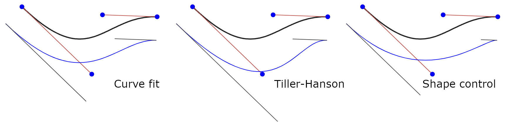
In addition to the accuracy for generating a single line segment, it is interesting to compare the scaling as the number of subdivisions increases, or as the error tolerance decreases. These tend to follow a power law. For this technique, it is $O(n^6)$, meaning that subdividing a curve in half reduces the error by a factor of 64. For the shape control approach, it is $O(n^5)$, and for Tiller-Hanson is is $O(n^2)$. That last is a surprisingly poor result, suggesting that it is only a constant factor better than subdividing the curves into lines.

The shape control technique has good scaling, but stability issues when the tangents are nearly parallel. That can happen for an S-shaped curve, and also for a U with nearly 180 degrees of arc.
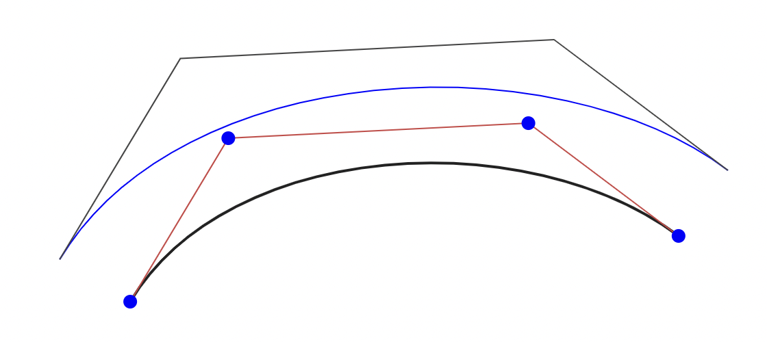
The Tiller-Hanson technique is geometrically intuitive; it offsets each edge of the control polygon by the offset amount, as illustrated in the diagram below. It doesn’t have the stability issues with nearly-parallel tangents and can produce better results for those “S” curves, but the scaling is much worse.
Regarding performance, I have preliminary numbers from the JavaScript implementation, about 12µs per curve segment generated on an M1 Max running Chrome. I am quite happy with this result, and of course expect the Rust implementation to be even faster when it’s done. There are also significant downstream performance improvements from generating highly accurate results; every cubic segment you generate has some cost to process and render, so the fewer of those, the better.
I haven’t implemented all the techniques in the Elber, Lee and Kim paper, but it is possible to draw some tentative conclusions from the literature. I expect the Klass technique (and its numerical refinement by Sakai and Suenaga) to have good scaling but relatively poor acccuracy for a single segment. The Klass technique is also documented to have poor numerical stability, thanks in part to its reliance on Newton solving techniques. The Hoschek and related (least-squares) approaches will likely produce good results but are quite slow (the Yang and Huang paper reports an eye-popping 49s for calculating a simple case with .001 tolerance, of course on older hardware).
The Euler spiral technique in my previous blog post will in general produce considerably more subdivision (with $O(n^4)$ scaling), but perhaps it would be premature to write it off completely. Once the curve is in piecewise Euler spiral form, a result within the given error bounds can be computed directly, with no need to explicitly evaluate an error metric. In addition, the cusps are located robustly with trivial calculation. That said, getting a curve into piecewise Euler spiral form is still challenging, and my prototype code uses a rather expensive error metric to achieve that.
Discussion
This post presents a significantly better solution to the parallel curve problem than the current state of the art. It is accurate, robust, and fast. It should be suitable to implement in interactive vector graphics applications, font compilation pipelines, and other contexts.
While parallel curve is an important application, the curve fitting technique is quite general. It can be adapted to generalized strokes, for example where the stroke width is variable, path simplification, distortions and other transforms, conversion from other curve representations, accurate plotting of functions, and I’m sure there are other applications. Basically the main thing that’s required is the ability to evaluate area and moment of the source curve, and ability to evaluate the distance to that curve (which can be done readily enough by sampling a series of points with their arc lengths).
This work also provides a bit of insight into the nature of cubic Bézier curves. The $O(n^6)$ scaling provides quantitative support to the idea that cubic Bézier curves are extremely expressive; with skillful placement of the control points, they can extremely accurately approximate a wide variety of curves. Parallel curves are challenging for a variety of reasons, including cusps and sudden curvature variations. That said, they do require skill, as geometrically intuitive but unoptimized approaches to setting control points (such as Tiller-Hanson) perform poorly.
There’s clearly more work that could be done to make the evalation more rigorous, including more optimization of the code. I believe this result would make a good paper, but my bandwidth for writing papers is limited right now. I would be more than open to collaboration, and invite interested people to get in touch.
Thanks to Linus Romer for helpful discussion and refinement of the polynomial equations regarding quartic solving of the core curve fitting algorithm.
Discuss on Hacker News.
References
Here is a bibliography of some relevant academic papers on the topic.
- An offset spline approximation for plane cubic splines, Klass, 1983
- Offsets of Two-Dimensional Profiles, Tiller and Hanson, 1984
- High Accuracy Geometric Hermite Interpolation, de Boor, Höllig, Sabin, 1987 (PDF cache)
- Optimal approximate conversion of spline curves and spline approximation of offset curves, Hoschek and Wissel, 1988 (PDF cache)
- A New Shape Control and Classification for Cubic Bézier Curves, Yang and Huang, 1993 (PDF cache)
- Comparing offset curve approximation methods, Elber, Lee, Kim, 1997 (PDF cache)
- Cubic spline approximation of offset curves of planar cubic splines, Sakai and Suenaga, 2001 (PDF cache)
- Boosting Efficiency in Solving Quartic Equations with No Compromise in Accuracy, Orellana and De Michele, 2020 (PDF cache)
- High-Performance Polynomial Root Finding for Graphics, Yuksel, 2022 (PDF cache)