Secrets of smooth Béziers revealed
I haven’t posted here much lately, and I admit, it’s because I’ve gotten sidetracked thinking about curves again. I did my PhD thesis on curves, so spent years thinking about them, then put that on hold for a while, aside from some work in crunching font file sizes down.
But a few weeks ago, Hrant Papazian tweeted at me a link to the paper on κ-Curves, which is what Adobe uses in the “Curvature Tool” in Illustrator, and that rekindled my interest.
I have always found Béziers unintuitive hard to learn to use well. That said, in expert hands they’re capable of quite smooth and expressive curves. I made a little interactive visualization that I think illustrates both of these, and perhaps gives some insight into how to use cubic Béziers to draw smooth curves.
To me, one of the smoothest curves is the Euler spiral. And, indeed, choosing the right metric (in this case, Minimum Curvature Variation), it can be proven to be the smoothest that fits the tangent constraints. The main focus of my Spiro work is that you should design curves using Euler spirals, then convert those to Béziers so they can be used in other software. Of course, as the κ-Curves paper points out, Euler spiral splines have some shortcomings, mostly that they don’t always have a unique solution, so they tend to “flip around” when moving control points, and Spiro’s solver is even less robust than that, sometimes flaking out and giving results that look like particle accelerator tracks.
But let’s say you have an Euler spiral and want to convert it into the closest possible cubic Bézier segment. I gave such an optimization algorithm in Chapter 9 of my thesis, but it didn’t give a tremendous amount of insight.
A good way to visualize the process of Bézier optimization is to run it for all possible Euler spiral segments, within a certain parameter range. So I dusted off my thesis code, and came up with this image:
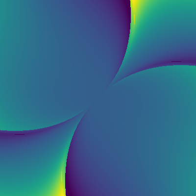
The horizontal axis is the tangent angle on the left side, the vertical axis is the tangent angle on the right side, and color represents the armlength, brighter is longer (using the viridis colormap). It’s not easy to explain, best to play with the interactive visualization instead. In that visualization, the accurate Euler spiral is plotted in red, the cubic Bézier on top in blue. Below that is a plot of curvature as a function of arclength.
Looking at this map, we see clearly that there are two domains. For anti-symmetrical cases (and symmetrical ones where the angles are not too close), the lower curvature side has the shorter arm, and the higher curvature side the longer one. But in the symmetrical domain it’s the other way around.
What’s perhaps most surprising is the behavior as it jumps from one domain to the other. The arm lengths change quite dramatically, but the curve very little. As arm lengths go to zero, you get these tiny cusps, where curvature goes very high, but the cusp is so tiny you don’t see it.
The optimizer also found a tiny domain where going all the way to zero arm lengths gives slightly better results than very short arm lengths, but this can safely be ignored. Again, though, it’s an example of how large changes to the control points can have subtle effects on the curve.
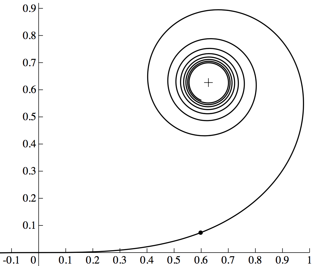
I now also have some insight into where exactly the jump between the two domains occurs: it’s when the center of the segment matches the Euler spiral at about t = 0.606, which I believe is the point where it most closely approximates a parabola. It might be interesting to explore more deeply exactly what’s going on there.
One way of thinking about this exploration is that cubic Béziers have a large parameter space encompassing both lumpy and smooth curves. The very smoothest are the ones that minimize the Minimum Curvature Variation functional, and we can plot all of them. This map tells you where to look to find them. Happy hunting!
Discuss on lobste.rs or Hacker News.