The stack monoid revisited

This is a followup to my previous post on the stack monoid, but is intended to be self-contained.

Motivation: tree structured data

GPUs are well known for being efficient on array-structured data, where it is possible to operate on the elements of the array in parallel. That last restriction doesn’t mean that the operations have to be completely independent; it’s also well known that GPUs are good at algorithms like prefix sum, where a simplistic approach would imply a sequential data dependency, but sophisticated algorithms can exploit parallelism inherent in the problem.

In piet-gpu, I have a particular desire to work with data that is fundamentally tree-structured: the scene description. In particular, there are clip nodes, described by a clip path, and whose children are masked by that clip path before being composited. The level of nesting is not limited in advance. In SVG, this is represented by the clipPath element, and the tree structure is explicit in the XML structure. All other modern 2D graphics APIs and formats have a similiar capability. For Web canvas, the corresponding method is clip, but in this case the tree structure is represented by the nesting of save and restore calls.

One of the design principles of piet-gpu is that the scene is presented as a sequence of elements. The tree structure is represented by matching begin_clip and end_clip elements. The problem of determining the bounding box of each element can be expressed roughly as this pseudocode:

stack = [viewport.bbox]
result = []
for element in scene:
    match element:
        begin_clip(path) => stack.push(intersect(path.bbox, stack.last()))
        end_clip => stack.pop()
        _ => pass
    result.push(intersect(element.bbox, stack.last()))

Basically, this represents the fact that each drawing element is clipped by all the clip paths in the path up to the root of the tree. Having precise bounding boxes is essential for the performance and correctness of later stages in the pipeline. There’s a bit more discussion in clipping in piet-gpu (an issue in this blog that hopefully will become a post soon).

The computation of bounding box intersections is not particularly tricky. If it were just a sequence of pushes and no pops, it could easily be modelled by a scan (generalized prefix sum) operation over the “rectangle intersection” monoid. The tricky part is the stack, which is basically unbounded in size. In my previous post, I had some ideas how to handle that, as the stack is a monoid, but the proposal wasn’t all that practical. For one, it required additional scratch space that was difficult to bound in advance.

Since then, I’ve figured out a better algorithm. In fact, I think it’s a really good algorithm, and might even be considered to push the boundary about what’s possible to implement reasonably efficiently on GPU.

For the remainder of this post, I’ll drop the bounding boxes and just consider the stack structure; those can be added back in later without any serious difficulty. This is known in the literature as the “parentheses matching problem” and has other names. I prefer “stack monoid” because identifying it as a monoid is a clear guide that parallel (or incremental) algorithms are possible, but I’m not sure the term has caught on. Another reason I prefer the “monoid” terminology is that it emphasizes that the pure stack monoid can be composed with other monoids such as axis-aligned rectangle intersection; conceptually I think of the data type implemented by this algorithm as Stack<T> where T: Monoid.

The simplified problem can be stated as:

stack = []
for i in 0..len(input):
    result.push(stack.last())
    match input[i]:
        '(' => stack.push(i)
        ')' => stack.pop()

Here, every open parenthesis is assigned the index of its parent in the tree, and every close parenthesis is assigned the index of its corresponding open parenthesis. Note that here I’ve also changed the order so that generating the result happens before processing the element. This is analogous to the distinction between inclusive and exclusive prefix sum; generally the same algorithm can be used for both, but sometimes one or the other is more convenient. When computing bounding boxes, the inclusive version is better, because we want the bounding box of the element, as modified by the clips. But for purely tracking tree structure, the exclusive version is easier.

An example:

index 0  1  2  3  4  5  6  7  8  9 10 11 12 13 14 15 16 17
input (  (  (  )  (  (  (  )  )  (  (  )  (  )  )  )  )  )
value -  0  1  2  1  4  5  6  5  4  9 10  9 12  9  4  1  0

It might be easier to visualize in tree form:

An interesting fact is that from this it’s quite straightforward to reconstruct the snapshot of the stack at each element, just by walking up the chain of parent links to the root. And, importantly, this “all snapshots” representation takes no more space than the stack itself (assuming the input has no additional bounds on nesting depth). This sequence-of-snapshots can be considered an immutable data structure which is gradually resolved and revealed by the algorithm, as opposed to the stack itself, which is both mutable and requires O(n) space for each instance, a serious problem for efficient GPU implementation.

The stack monoid, restated

In case this “monoid” language is too confusing or abstract, there’s a more concrete way to understand this, which will also be useful in explaining the full GPU algorithm. Consider the snapshot of the stack at each iteration of the above simple loop. Then it turns out to be fairly straightforward to express a command to go from the stack at step i to the stack at step j: pop some number of elements, then push a sequence of some new ones.

That command is a monoid. It has a zero: pop 0 and push the empty sequence. Each input can be mapped to this monoid: a ‘(‘ at position i is just pop 0 and push [i], and ‘)’ is pop 1 and push nothing. And the magic is that any sequence of two can be combined. There are two cases, depending on whether the push of the first is larger or smaller than the pop of the second. Here expressed in pseudocode:

fn combine(a, b):
    if len(a.push) >= b.pop:
        return { pop: a.pop, push: a.push[0 .. len(a.push) - b.pop] + b.push }
    else:
        return { pop: a.pop + b.pop - len(a.push), push: b.push }

The ability to compute the stack monoid on slices of the input, then stitch them together later, is essential for processing this in parallel. Otherwise it would be very hard to do better than purely sequential processing.

In-place reduction

My previous blog post suggested a window of size k with a spill feature. No doubt this can be done, but dealing with the spills would be quite tedious to implement and also use extra scratch memory that’s hard to bound.

The solution is to do the reduction in-place. Before, there are two monoid elements derived from input slices of size k each, and after, there is one covering an input slice of size 2 * k. The key insight is that shuffling the monoid can be done in-place, requiring 1 step of 2 * k parallel threads.

The details of the accounting are slightly tedious, but conceptually it’s simple enough. It helps when the sequence is right-aligned; note that all elements in b’s push sequence are preserved, so nothing needs to happen. If there is one thread per element, as is typical in a GPU compute shader workgroup, each thread just decides its value, based on the push and pop counts of the two inputs: either empty (in which case it doesn’t need to be written), or a value from one of the two input sequences. It’s probably easiest to show that as a picture:

Then, for a workgroup of, say, size 16, it’s possible to compute the stack monoid for that workgroup in a tree of 4 stages:

Note that these stack slices are not the final output. Rather, they are intermediate values used to compute the final output. In general, when doing a combination of two stack slices (monoid elements), some of the outputs in the second slice can be resolved. For example, when combining a single push and a single pop, the output corresponding to the pop element is the index of the push, but the resulting stack slice is empty. When parentheses are matched in this manner, they are recorded to the output then erased from the resulting stack slice. In other cases, the outputs are still pending, and wait for a later combination. This generation of the output is not shown in the figures above, but features prominently in the code.

Look-back

The central innovation of this algorithm is using decoupled look-back to stitch the stack segments together and resolve references that cross from one partition to another. At the end of the partition-local reduction, so at the beginning of the look-back phase, each partition has published its own monoid element. At the end of the look-back phase, each partition has a window of the snapshot of the stack, the size of the window matching the partition size. Then, all outputs for a partition can be resolved from that window.

This idea of a snapshot of size 1024, every 1024 elements (to pick a typical partition size) is key. The total storage required is also one cell per input element, same as the purely sequential case. And by having a slice rather than a single link, a workgroup can process all elements in the slice in parallel.

The algorithm is layered on top of decoupled look-back. It’s worth reading the paper to get a detailed understanding of the algorithm, and especially why it works well on modern GPUs (it’s not obvious), but I’ll go over the basic idea here. In the simplest form, each partition is in three states: initial, it has published its local aggregate (using only information from the partition), or it has published the entire prefix from the beginning. A partition walks back sequentially and proceeds depending on the state. If it’s still initial, it can make no progress and spins. If it’s a local aggregate, it does the monoid operation to add it, then continues scanning. And if it hits a published version, it incorporates that, publishes the result, and is done.

This almost solves the problem, but there is one remaining detail. It’s possible that, even when you reach a published prefix, the stack slice that results from combining with it is smaller than the partition size. This will happen when the stack itself is larger than the partition (so would not happen if the maximum stack depth were bounded by the partition size) and the second monoid element has more pops than pushes. The solution is to follow the link from the bottom of the stack slice published by the leftmost scanned partition. This is a generalization of following the chain of parents as described earlier, but because the stack slice is (typically) 1024 elements deep, following the bottom-most link allows jumping over huge chunks of the input. In testing with random parentheses sequences, the algorithm seldom if ever needed to follow more than one such backlink, and following the backlinks at all (which could be suppressed by bounding input stack depth) only added a few percent to total running time. A slight caution: an adversarial input could probably force resolution of a potentially large number of backlinks.

Some theory

Back in the early ’90s, it was trendy to come up with parallel algorithms for problems like this. At the time, it wasn’t clear what massively parallel hardware would look like, so computer scientists mostly used the Parallel RAM (PRAM) model.

After publishing my stack monoid post, a colleague pointed me to the PRAM literature on parentheses matching, and in particular I found one paper from 1994 that is especially relevant: Efficient EREW PRAM algorithms for parentheses-matching. In particular, the in-place reduction is basically the same as their Algorithm II (Fig. 4). Sometimes studying the classics pays off!

The PRAM model is good for theoretical analysis of how much parallelism is inherent in a problem, but it’s not a particularly accurate model of actual GPU hardware of today.

A detailed theoretical analysis of the algorithm I propose here is tricky, for a number of reasons. An adversarial input can force following a chain of backlinks up to the size of the workgroup, though I expect in practice this will almost never be more than one. Analysis is further complicated by the degree of look-back. However, there is one simple case: when the stack is bounded by the workgroup size, there is never a backlink, and thus the analysis is basically the same as decoupled look-back. Since the workgroup size is typically 1024, for both parsing tasks and 2D scene structure, it’s plausible it will never be hit in practice. Even so, randomized testing suggests the algorithm is still very efficient even with deeper nesting.

Other older literature that’s relevant is section 1.23 (ordered trees) in Iverson’s APL book. Generally this requires a matrix proportional to the number of elements times the maximum depth, but perhaps could be useful as the basis for other, more space-efficient algorithms. A particularly intriguing direction is Aaron Hsu’s thesis on co-dfns, which has data structures similar to this post, though generally prefering a depth-first rather than breadth-first sort of the input elements.

More on memory coherence

Part of the development of this algorithm was revisiting memory coherence, as I had some nasty bugs on that front. I was able to resolve them in a satisfactory way.

When I explored implementing prefix sum, my attempt at a compatible solution was to put the volatile qualifier on the buffer used to publish the aggregates. And that worked in my testing in Nvidia GTX 10x0 GPU’s. I was hopeful that, while not properly specified anywhere, accesses to a volatile buffer would implicitly have acquire and release semantics, as was the case in MSVC. However, this was unsatisfying, as “it works on one GPU” is a weak guarantee indeed.

My feeling at the time was that the Vulkan memory model was the best way forward, in that it gave a precise contract between the code and the GPU; the code can ask for exactly the level of memory coherence required, and the GPU can optimize as aggressively as it likes, as long as it respects the constraints. The current version of the prefix sum implementation requires the Vulkan memory model extension.

The problem with that is portability: Vulkan is the only API that allows explicit fine-grained memory semantics, in particular separating acquire and release, rather than just having a barrier that implies both, and even there the feature is optional. Other APIs provide relaxed atomics only.

Experimentation shows that volatile alone is indeed not sufficient, and on other GPUs it is possible to observe reordering that breaks reliable publishing. Fortunately, I believe there is a way forward; using the coherent qualifier on the buffer, and placing an explicit memoryBarrierBuffer() call before a release store or an acquire load.

Shader language abstractions have an opportunity to fix this. It would be very nice to specify desired memory semantics very precisely, as in the Vulkan memory model, and have that compile to the target API. If recent Vulkan is available, it’s a direct mapping. Figuring out the exact translation to other APIs is not easy, partly because documentation is sparse; it really requires detailed insider knowledge of how these other GPUs work. See gpuweb#1621 for a bit more discussion. I believe WebGPU is the most promising place for this work, but it’s also tricky and subtle for a variety of reasons (lack of good documentation of existing APIs being one), so I expect it to take some time. There are other potential efforts to watch, including rust-gpu. In any case, I would consider ability to run decoupled look-back to be a benchmark for whether a bit of GPU infrastructure can run reasonably ambitious compute workloads.

Another thing to note is that the current prototype, while otherwise portable, can get stuck because the GPU may not offer a forward progress guarantee. There is code (thanks to Elias Naur) in piet-gpu to guarantee forward progress in this case, basically a scalar loop that slowly makes progress in what would otherwise be a spinlock, and similar logic is needed here too.

Performance

One of the most important things about having working code is that it’s possible to measure its performance. Testing that it’s correct is also important, of course!

I measured this implementation on an AMD 5700 XT, which is a reasonably high end graphics card, though not top of the line. The bottom line performance number is 2.4 billion elements per second (the test was processing a sequence of 1M pseudorandom parens). This is about 10x faster than the Rust scalar code to verify the result. I would characterize this as pretty good but not necessarily jaw-dropping. You probably wouldn’t want to upload a dataset to the GPU just to match parenthesis, but if you can integrate this into a pipeline with other stages and keep the data on GPU rather than doing readback to the CPU, it’s potentially a big win.

It’s instructive to break down the performance and see how it varies with workgroup size. In the following chart, I measured the time for just the local reduction, and also the full algorithm including look-back.

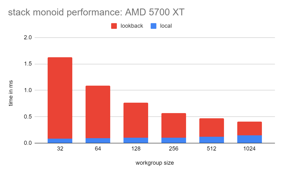
The time for the local reduction is proportional to lg(workgroup size), and measurement of that is as expected. The cost of the look-back decreases as the workgroup size increases, which is not surprising - the total number of publish operations needed is inversely proportional to the workgroup size. Since (in this implementation) look-back is more expensive, the best performance is at a workgroup size of 1024. A larger workgroup might be slightly better, but looking at this graph, not dramatically so.

This implementation uses a relatively simple sequential approach to the look-back. It is based on my prior prefix sum implementation, in which I was able to avoid that being the performance bottleneck by pushing the size of the workgroup (each thread processed 16 elements, for a workgroup size of 16k elements; typical GPUs have a limit of 1024 threads per workgroup). It is likely possible to increase the size of the workgroup by iterating multiple elements per thread, but not necessarily easy; shared memory would quickly become the limiting factor, as this algorithm requires shared memory for the stack, while in a pure prefix sum the monoid results can mostly be stored in registers. Thus, I think the best prospect for further improving performance is parallelizing the look-back, as suggested in the original paper.

I also experimented with other potential optimizations. I tried using subgroups for the local reductions, but did not see an improvement. It’s possible that (non-uniform) subgroupShuffle()has poor performance characteristics on AMD. I also tried a two-pass tree reduction without look-back, and that gave somewhat encouraging results: it was almost twice as fast as the look-back implementation, but limited to (partition size)^2 elements, ie about a million. I strongly suspect this performance gain would evaporate with more passes to overcome the size bound.

Of course, it’s also possible there could be algorithmic improvements; I would count this implementation as moderately work-efficient, with a work factor of at least lg(workgroup size) for the local reduction. The PRAM literature suggests a more theoretically work-efficient algorithm is possible, but it’s also quite plausible that wouldn’t translate to an actual performance gain due to extra complexity - my experience in GPU so far strongly suggests that simpler is better.

As mentioned above, changing the input to bound the stack depth has only a minor performance bump, giving evidence that the cost of following the backlinks (and thus enabling completely unbounded stack depth) is not significant. In fact, this algorithm can smoothly handle sequences with very deep nesting, which can be problematic for other implementations. For example, it can trigger stack overflow in a recursive descent parser.

Overall, I am happy with the current performance, as I think clip stack processing will barely show up in profiles of the full piet-gpu pipeline. Keep in mind that soft clipping is traditionally one of the most expensive operations in traditional approaches to 2D rendering, especially on GPU where it usually entails allocating scratch buffers to render the mask and do the compositing.

Conclusion

I have long been interested in problems where GPUs need to efficiently process data that has a tree structure in some form. My explorations into the stack monoid strongly suggested that an efficient GPU implementation was possible, but until now I did not have a practical algorithm.

The main ingredients for the algorithm, on top of the theoretical insight offered by the stack monoid (and classic CS literature in parallel algorithms) are: in-place reduction of the monoid (meaning that scratch memory is tightly bounded), representation of the stack snapshots as partition-sized slices, and a careful attention to doing as much as possible within a workgroup. This algorithm also layers on top of the excellent decoupled look-back approach, which allows the use of a single pass and thus avoids extra memory traffic for re-reading the data in multiple passes.

The algorithm turned out well, with reasonably straightforward implementation (by GPGPU standards, anyway) and good performance. Likely more improvements are possible, but I think it’s plenty good enough as-is to serve as the basis for a new clip stack implementation in piet-gpu.

It is likely there are other practical applications. The main motivation for theoretical work has been parsing, and I think this algorithm could serve as the basis for a parser for a tree-structured format such as JSON.

Thanks to Elias Naur for advocating improvements in the current handling of clip bounding box handling in piet-gpu.

There’s a bit of discussion on lobste.rs.