How long is that Bézier?
One of the fundamental curve algorithms is determining its arclength. For some curves, like lines and circular arcs, it’s simple enough, but it gets tricky for Bézier curves. I’ve implemented these algorithms for my new kurbo curves library, and I think the work that went into getting it right makes a good story.
Béziers and arclength
First, if you haven’t read A Primer on Bézier Curves, go do that now. In particular, the section on arclength motivates almost everything I’m writing about below.
Why is arclength important? One important traditional application is rendering strokes with dashed patterns. My main interest is part of generating optimized Béziers to closely fit a given curve. My research has shown that the optimum Bézier tends to have an arclength very close to the original curve. Thus, searching only for Béziers with matching arclength is a good way to reduce the parameter space when searching for optimum fit. I use this technique in the Euler explorer, as well as optimized conversion from Spiro to cubic Béziers in my PhD thesis. I’m embarrassed to admit, though, that the code I used for that is very slow and not all that precise — generating the full map for the Euler explorer took hours.
The most obvious approach to computing arclength is to sample the curve at a sequence of points, then add up all the distances. This is equivalent to flattening the curve into lines and adding up all the line lengths. It’s simple and robust (it doesn’t care too much about the presence of kinks), so fairly widely implemented. The only problem is, it’s not very accurate. Or, to put it another way, it’s astonishingly slow when high accuracy is desired. The accuracy quadruples with every doubling of the number of samples, or another way of putting it, the number of samples is $O(\sqrt{N})$ where $N$ is the reciprocal of the error tolerance.
Let’s try to find a better way. This question was posed on Stack Overflow, specifically for quadratic Béziers, so to a large extent this post is an extended answer to that question, though we will also give a solution for cubic Béziers.
For a parametric curve, expressed as $x(t)$ and $y(t)$, where $t$ ranges $(0..1)$, the arclength of a curve is this integral:
\[\int_0^1 \sqrt{(dx / dt)^2 + (dy / dt)^2}\ dt\]For quadratic Béziers, this integral has a closed form solution. I tried implementing the arsinh-based formula in the Stack Overflow post, and couldn’t get it to work. Also, I was both aware that cubics don’t have a closed form solution, and worried about numerical stability (rightfully so, as we’ll see below), so went down the path of adaptive subdivision algorithms.
The control polygon length approach
In that Stack Overflow post was a reference to “Adaptive subdivision and the length and energy of Bézier curves” by Jens Gravesen. My first step was to implement that. Long story short, it’s not terrible, but it is possible to do better.
The insight of the Gravesen paper is that the actual length is always somewhere between the distance between the endpoints (the length of the chord) and the perimeter of the control polygon. And, for a quadratic Bézier, 2/3 the first + 1/3 the second is a reasonably good estimate.
More to the point, Gravesen’s approach gives hard error bounds, which is the basis of a subdivision approach. At each step, you test whether the estimate is within the desired tolerance. If so, you use the approximation. If not, you subdivide (using de Casteljau, of course), and run the algorithm on each half. This metric has 1/16 the error for each subdivision, so we’re at $O(N^\frac{1}{4})$ worst case, decidedly better than above.
Gravesen also observed that the approximation is often a lot better than the error bound would indicate. When this happens, successive refinements don’t change the estimate much. Why not use the amount by which the estimate changes on subdivision as a more realistic bound? Gravesen observes, “Error estimate no. 1 overestimates the error, and there are up to 400 times too many subdivisions. Error estimate no. 2 seems to be reliable…” And several examples are given in which it does the right thing. Much of the paper is taken with theorems and proofs that the error bound is accurate, so I thought I was on solid ground.
Empirical evaluation
The section on arclength in the Primer suggests Legendre-Gauss quadrature. After implementing the Gravesen algorithm, of course I wondered, is that better? How much so?
The best way to evaluate such questions is to visualize the data. It would be nice to plot an error metric for every possible quadratic Bézier. That might seem tricky, but it turns out that quadratic Bézier curves can be considered a 2-parameter curve family. For any arbitrary quad segment, translate, uniformly scale, and rotate the curve to bring the endpoints to fixed positions. These operations (known as conformal transformations) don’t affect the fundamental shape of the curve, and arclength measurement should be invariant to them.
For this evaluation, it’s convenient to put the endpoints at (-1, 0) and (1, 0). Then, the two free parameters can be interpreted simply as the control point in the middle. The reason for these particular points is that the center point can be interpreted as the second derivative of the curve. When it’s at (0, 0) it’s a straight line, which is especially easy. Also, the more a curve is subdivided, the closer the subdivided curves come to a straight line.
Here’s what such a map looks like; smooth Béziers near the bottom left corner (which is 0,0), more curved ones farther out, up to 2 in each direction. Along the bottom edge, up to (1, 0) are straight lines just with the control point shifted, but beyond that are pathological curves that contain an infinitely sharp turn; not surprisingly, these will be tricky for some algorithms.
Given such a map of all possible quadratic Béziers, we can now plot the accuracy of various approximate algorithms. Here’s the Gravesen one:
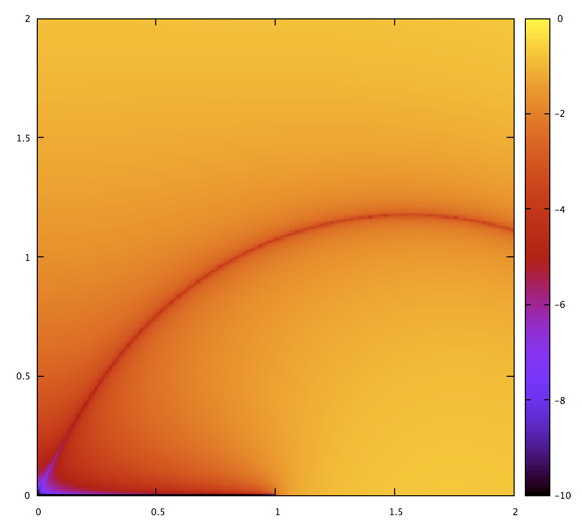
This is plotted as error on a log-scale. Black and blue are the most accurate (10 and 8 digits of precision), 0 the least. Not surprisingly, we see it do well for nearly straight curves. There’s also a line in the middle, but there’s nothing special about it; it’s just a visual indication that the approximation overshoots on one side and undershoots on the other, so the error happens to be 0 between those two regions.
Now to compare to Legendre-Gauss quadrature. Fortunately there’s code for that in Pomax/BezierInfo-2#77 by Behdad so it was easy enough to test.
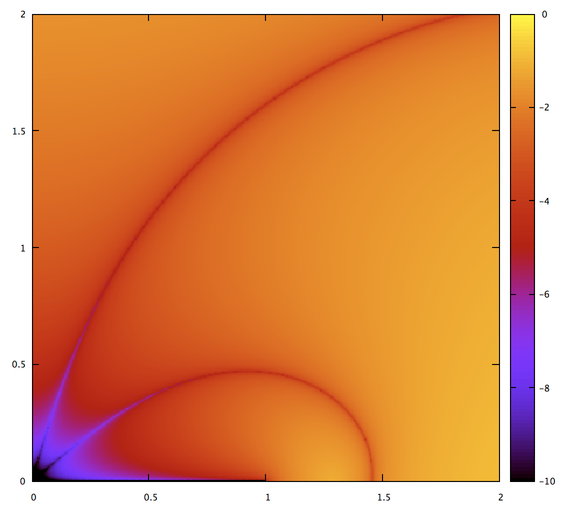
It’s quite a bit better; the region where it’s very accurate is bigger. Interestingly enough, though, it doesn’t do a lot better for extreme cases. Intuitively, it should be possible to get accurate results with fewer subdivisions. The problem is: how do you compute a bound on the error? The advantage of the Gravesen approach is that it has the error metric built-in.
Or does it? Let’s verify that. I implemented the adaptive subdivision from the Gravesen paper and then made this plot, with the accuracy threshold set to 1e-4:
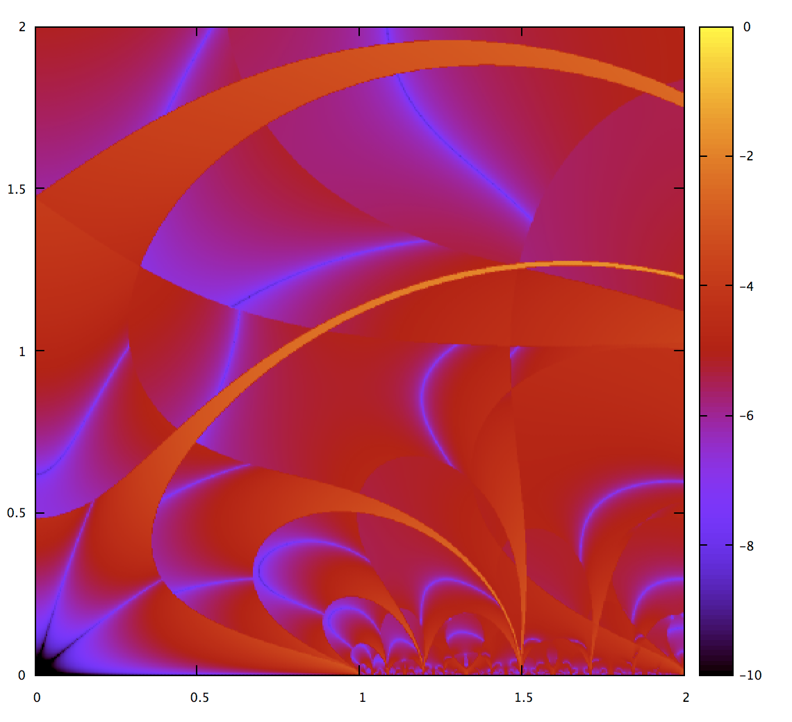
If it’s working as intended, then no part of the map should go beyond red, the color for 1e-4. But we can see that for some stripes (generally the regions where the approximation is crossing from overshoot to undershoot), the error is underestimated as well, and there are bits of orange where that happens. It’s a fairly small fraction of the area of the map, and these get even thinner as the threshold is set lower. But even so, as a way to guarantee measurements of a given accuracy, it’s a failure. We need a better approach.
(I’m using the arclen_accuracy example program in kurbo to make the raw data for these plots, then gnuplot with mostly default settings to visualize them.)
Incidentally, this map also lets us visualize the subdivisions; they’re sharp lines with the choice to subdivide or not subdivide on either side.
Quadrature overkill
How does Pomax’s Bezier.js solve this problem? Looking at the code, it uses 24-order Legendre-Gauss quadrature. This seems like it should be massive overkill and is not that expensive to compute (it’s basically 24 “hypot” operations plus some linear math). Can we just do that? Let’s take a look.
Looking at this, reasonably smooth quadratic Béziers get measured very precisely, but more extreme ones do not. In fact, for the ones that have sharp kinks, it only does a little better than the simpler techniques. So it’s overkill for part of the range, and undershoot for other parts. These pathological Béziers can and do happen, especially during interactive editing. For completely general use, the technique in Bezier.js doesn’t solve our problem.
Incidentally, if I ever start a punk band, it will be called “quadrature overkill.”
An error metric
One way to move forward is to cook up an error metric that absolutely bounds the error of some approximation. Ideally this metric is fairly tight, otherwise it’ll tell us we need to subdivide when we don’t. I basically came up with one by “painting with math”. It’s just a 2-parameter function, and we know the general shape it needs to have just by looking at the images. For the 3rd order quadrature above, I came up with this function:
let est_err = 0.06 * (lp - lc) * (x * x + y * y).powi(2);
Here the lp and lc variables represent the length of the perimeter and chord; these ideas are borrowed from the Gravesen paper, and including that gives us a tighter bound for values near the bottom edge of our plot. Other than that, it’s basically the norm of the second derivative raised to the power that matches the scaling of our quadrature.
One good way to validate such a function is scatter plots; for each point we plot the estimated error on the x axis, and the actual error on the y axis. No point is allowed to be above the x=y line, and ideally every point is pretty close to it. Let’s see how we did:
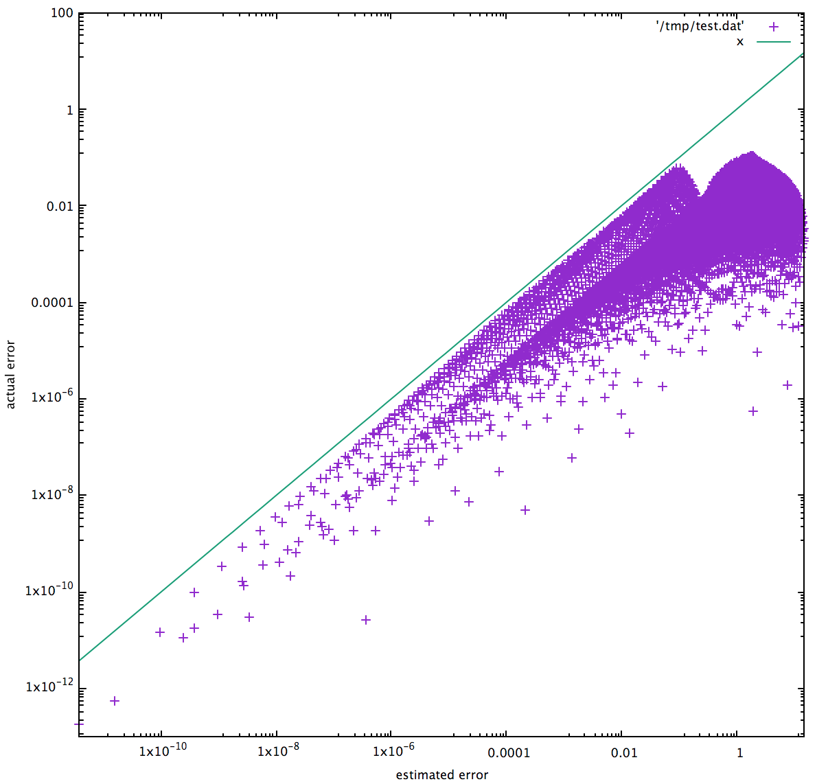
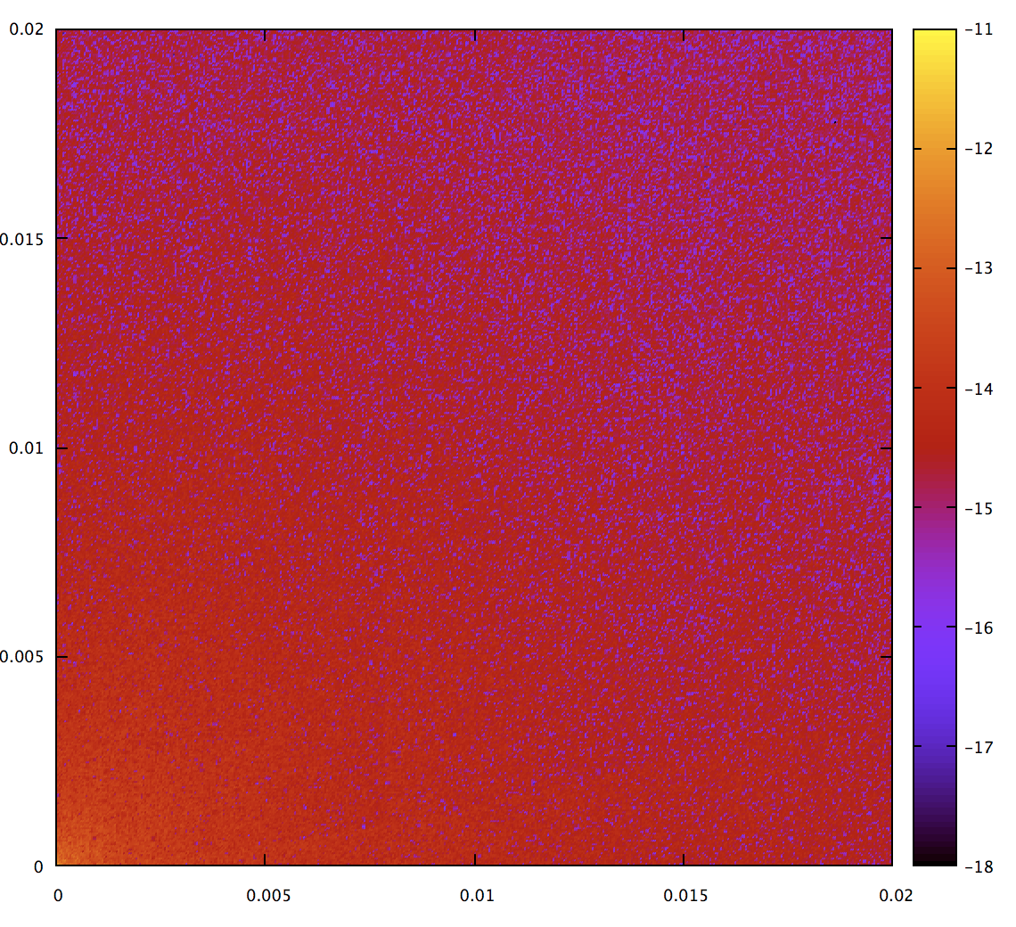
That’s a good error metric. And let’s see how it performs:

Note that the colors are rescaled; it only goes up to 1e-4 so we can see more clearly (and because it’s prettier that way). And we see that the metric is doing well; precision much better than the threshold is a sign we’re wasting computation. We also see that it’s subdividing less than the Gravesen metric, which means computation is faster.
Back to analytics
I sent some of this to Pomax, who reminded me that the arclength of a quadratic Bézier has a closed-form analytical solution. If I’m going for the best possible solution, shouldn’t I give that another try? And honestly, by this time my competitive spirit had kicked in. If there was a better solution for this problem than what I had in kurbo, I wouldn’t be happy.
I’m not going to go over the solution of the integral, fortunately Mateusz Malczak has written up a good explanation, and it comes with working code as well. And who integrates things by hand any more? If the integral is at all tractable, just put it into Mathematica and it’s almost certain to find it. This is what Mateusz came up with:
\[\frac{1}{8a^\frac{3}{2}}{\Large[}4a^\frac{3}{2}\sqrt{a+b+c}+2\sqrt{a}b(\sqrt{a+b+c} - \sqrt{c}) - (b^2 - 4ac)\ln{\large |}\frac{2\sqrt{a} + \frac{b}{\sqrt{a}} + 2\sqrt{a+b+c}} {\frac{b}{\sqrt{a}} + 2\sqrt{c}}{\large|} {\Large]}\]Easy! In this formula, $a$, $b$, and $c$ represent squared norms of the second and first derivatives at $t=0$, and $c$ is the squared norm of chord length. Details are of course on the linked page.
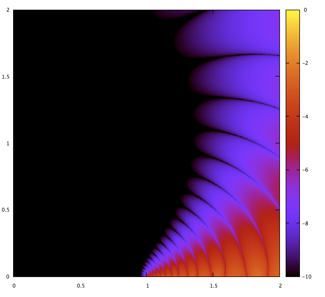
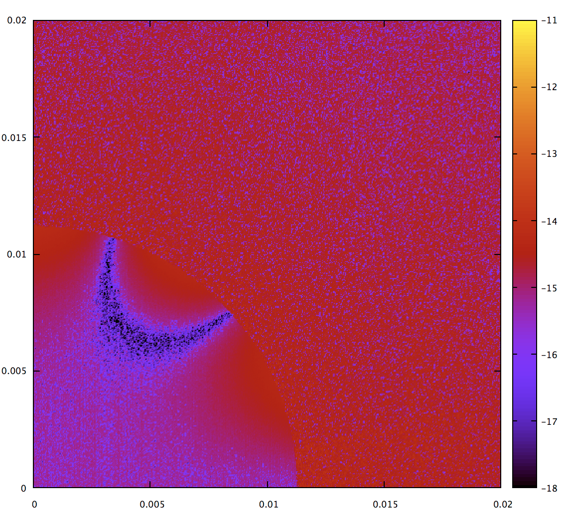
I had several concerns about this approach. One is numerical stability; the formula has several divide operations, which mostly are mostly over powers of the second derivative norm. Given that, it’s likely that accuracy will degrade as the curve gets closer to a straight line. And inded, for an exact straight line this code gives NaN. Zooming in, we can see the problem:
Note that the colors are rescaled again; the worst error on this map (other than the NaN at the origin which is not plotted) is 1e-11. That’s not bad, but let’s do the best we can while fixing the singularity at the origin. Fortunately, already have a function which is good in that range, the quadrature approach. The actual code in kurbo compares the second derivative norm against a threshold, and switches to quadrature inside that:
There’s another numerical instability for curves with a sharp kink (surprise, surprise); internal to the math this happens when $b^2 - 4ac$ becomes zero. It’s fixed in a similar way. Also, in addition to the visualizations in this blog post, kurbo has tests for these cases. I believe this algorithm has over 13 digits of precision over the entire map.
Performance
Does the extra accuracy of the analytical approach (with the fixes in place for numerical stability) come at a cost? Let’s benchmark:
test bench_quad_arclen ... bench: 46 ns/iter (+/- 17)
I’m impressed. It’s quite a bit faster (21ns) without the numerical stability fixes and with target-cpu=native, but for a library I think it’s much more important to be robust than absolutely at the edge of performance.
Onward to cubics
Of course, the analytical solution is only applicable to quadratics. The Abel–Ruffini theorem proves that it can’t be solved in closed form for higher polynomials. So for cubics we go back to the adaptive subdivision approach.
Again, the tricky part is the error metric. The error metric for a quadratic Bézier is based on the norm of the second derivative. For a quadratic, the second derivative is constant, so it’s easy to write expressions in terms of it. For a cubic, the second derivative is linear in $t$, so we want to somehow capture the fact that it varies across the parameter space.
Unlike quadratics, it’s hard to visualize the space of all possible cubics; it’s a four-parameter space, and my ability to visualize fields in four dimensions is limited. Thus, instead of 2d maps I mostly used randomly generated cubics, and scatterplots of whatever I wanted to measure from those. Cubics are also trickier, it’s not going to be easy to get error bounds as tight.
After some experimentation, mostly iterating on those scatter plots and trying things that either improved the tightness of the error bound or made it worse, I found that working with the integral of the second derivative norm was both tractable and gave a decent error bound.
Let’s write the second derivative as a simple linear equation:
\[cubic''(t) = at + b\]Then we want the integral of its square across the parameter range:
\[\int_0^1 (at + b)^2 dt\]Since this is just a polynomial, and doesn’t have a square root in it, the integral is nearly trivial: it’s $|a|^2/3 + a \cdot b + |b|^2$. I even did this without using Mathematica :).
It’s also nice that this is easy to compute; I tried approaches based on numerically integrating a more sophisticated error metric, but then the time spent computing the metric dominates the time actually approximating arc length.
All this work is based on heuristics. Going to higher order quadrature helps up to a point, but as long as we’re able to estimate the error metric accurately enough. I found a good compromise with a 9th order quadrature.
There are a few ways to evaluate performance. One is a scatterplot of the number of subdivisions required and the actual accuracy. Below is a sampling of random cubic Béziers with an error tolerance of 1e-4:
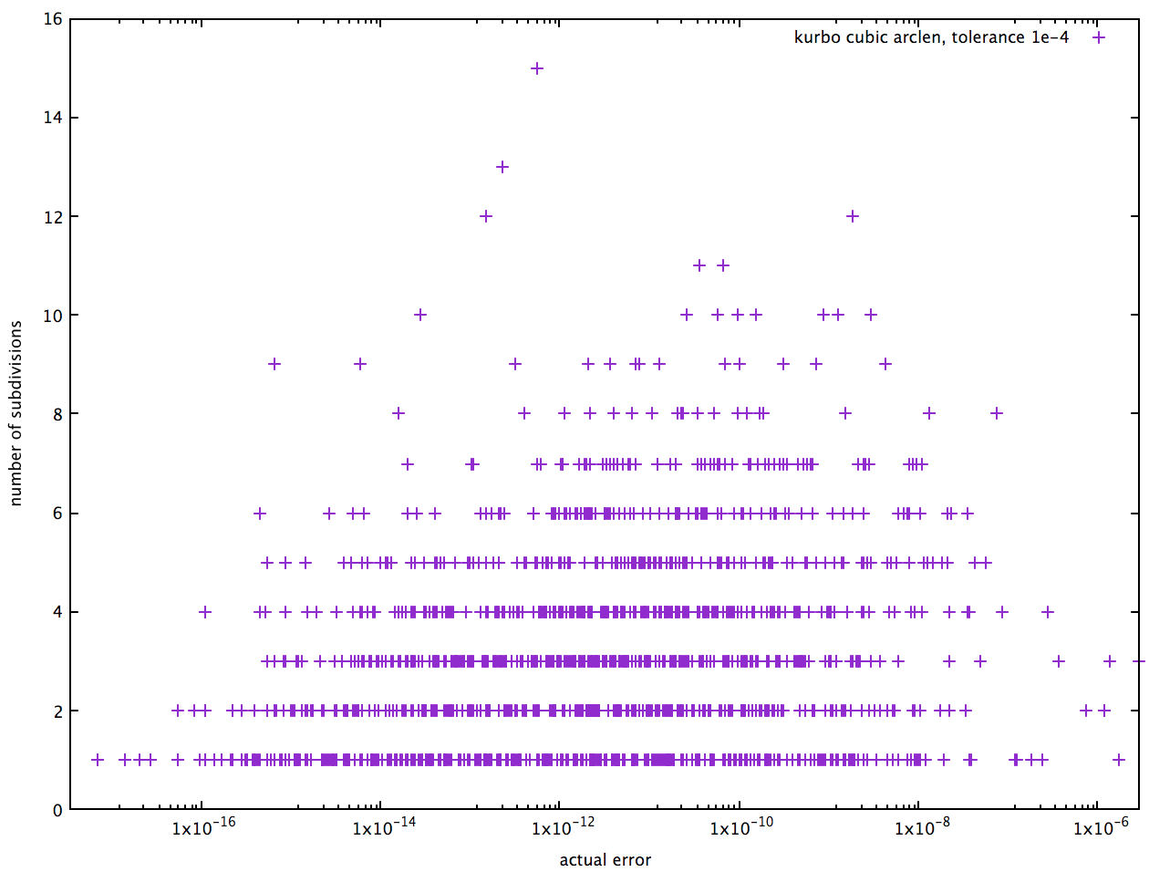
The vertical axis has the number of subdivisions, and the horizontal axis the actual error. Obviously we don’t want any points to the right of the specified tolerance. The majority of cases are handled with 4 or fewer subdivisions (in fact the mean is about 3.4 over my sample). It would be nicer to have them bunched closer to the right, but that would require a better error bound. Perhaps some enterprising reader will take up this work :).
We can benchmark the time taken as well:
test bench_cubic_arclen_1e_4 ... bench:         231 ns/iter (+/- 98)
test bench_cubic_arclen_1e_5 ... bench:         206 ns/iter (+/- 93)
test bench_cubic_arclen_1e_6 ... bench:         423 ns/iter (+/- 114)
test bench_cubic_arclen_1e_7 ... bench:         424 ns/iter (+/- 160)
test bench_cubic_arclen_1e_8 ... bench:         634 ns/iter (+/- 267)
test bench_cubic_arclen_1e_9 ... bench:         631 ns/iter (+/- 161)
While not quite as impressive as the quadratic case, these are still good showings and should be quite fine for production use. The Bézier benchmarked here is (0,0), (1/3, 0), (2/3, 1), (1,1), which has a nice “S” shape; computation time is dependent on the shape, and of course pathological Béziers with kinks will need more subdivision.
Lessons learned
I enjoyed this journey; it was a chance to dive deep into territory I find fun. I feel it’s likely that kurbo now has the finest arclength measurement code of any curves library on the planet. If anybody knows of better, please let me know! It’s likely that many other libraries have ranges where they give inaccurate results (especially for pathological Béziers) and are likely not as performant.
I also found Rust to be an excellent implementation language for this work. I enjoyed writing code using higher level concepts and being able to rely on the compiler to flatten out all the abstraction and generate excellent code (in a few cases I looked at the asm, it’s pretty sweet).
One lesson is to always empirically measure what you’re doing. Guaranteed you will learn something, otherwise you’re flying blind. Visualizations are especially good because you can see lots of data points. Similarly for randomly generated data. Otherwise there’s a good chance you’ll miss something.
This is especially true when working from academic papers. Having lots of theorems is not a reliable sign the algorithms translate directly to robust code.
Another lesson is that simpler curves such as quadratics are easier to work with and ultimately give better results in spite of needing more of them to accurately represent a curve. I found this holds for the nearest point method; for quadratics there’s an exact solution based on solving a cubic equation, but cubics require subdivision. I suspect the same will be true of other algorithms including offset curve.
Other resources
Behdad has a great TYPO Labs 2017 presentation on the math used for variational fonts. The implementation of arclength in FontTools uses the same basic analytical approach, and this is shown in the video along with low-order Legendre-Gauss Quadrature and recursive perimeter-chord subdivision. The presentation also shows exact calculation of area using Green’s theorem (also implemented in kurbo) and the use of SymPy to compute curve properties symbolically.
Jacob Rus has an interactive Bézier Segment Arclength Observable notebook. It uses high-degree Chebyshev polynomials, which are closely related to Legendre polynomials, and there’s a sophisticated inverse solver (needed for dashing). The inverse solver in kurbo is bisection, which is robust but not as fast in smooth cases.
Future work
I think arclength of quadratics is pretty much settled at this point. For cubics, the current solution is pretty good, but can likely be improved a bit more. Certainly I make no claims the error metric is perfect, and a tighter bound on that would unlock exploiting higher degree quadrature, which could converge a lot faster. One promising approach is to identify problematic inputs (ones for which the actual error is worse than what a simplistic error metric would predict). If, as seems likely, curves with cusps are an important category of those, then using the Stone and DeRose geometric characterization could help find those (thanks Pomax for the idea). Another idea (thanks to Jacob Rus) is to search for curvature maxima and use that to guide the subdivision. Determining maximum curvature (at least approximately) should be fairly tractable, but as always there’s a tradeoff between the cost of computing the error metric vs the savings in subdivision.
Applying a Newton method is likely to speed up the inverse method. That shouldn’t be too hard.
Perhaps an enterprising math enthusiast will be inspired to take up these problems. If so, I’ll happily incorporate the work into kurbo.
I personally am inclined to declare victory and move on. There are other interesting curve problems to solve!
Thanks
Thanks to Pomax for the primer, Legendre-Gauss quadrature resources, and encouraging me to write this blog, as well as some feedback. Thanks to Behdad for the shared intellectual curiosity about Bézier math and the application to fonts, plus resource suggestions. Thanks to Mateusz Malczak for his derivation of the analytical quadratic Bézier arclength formula and permission to adapt his code. Thanks to Jacob Rus for feedback and suggestions.
And thanks to you for reading!
Discuss on lobste.rs and Hacker News.