Fitting cubic Bézier curves

Cubic Béziers are by far the most common curve representation, used both for design and rendering. One of the fundamental problems when working with curves is curve fitting, or determining the Bézier that’s closest to some source curve. Applications include simplifying existing paths, efficiently representing the parallel curve, and rendering other spline representations such as Euler spiral or hyperbezier. A specific feature where curve fitting will be used in Runebender is deleting a smooth on-curve point. The intent is to merge two Béziers into one, which is another way of saying to find a Bézier which best approximates the curve formed from the two existing Bézier segments.

In spite of the importance of the curve-fitting problem and a literature going back more than thirty years, there has to date been no fully satisfactory solution. Existing approaches either fail to consistently produce the best result, are slow (unsuitable for interactive use), or both.

The main reason the problem is so hard is a basic but little-known fact about cubic Béziers: with C-shaped curves (no inflection point and a small amount of curvature variation) there tend to be three sets of parameters that produce extremely similar shapes. As a result, in general when fitting some arbitrary source curve, there are three local minima. Approaches based on iterative approximation (in addition to being slow) are likely to find just one, potentially missing a closer fit of one of the others.

How close are two curves?

Before getting into the solution, we’ll need to state the problem more carefully. The goal is a cubic Bézier that minimizes some error metric with respect to the source curve. But how do we measure the distance between two curves?

One meaningful metric is the Fréchet distance. It can be explained with a little story. An aircraft engineer goes on a walk with their dog Pierre, and the path followed by each can be described by a curve. What is the minimum length leash that allows both to complete their paths? That is the Fréchet distance.

Also note that the Fréchet distance is closely related to the Hausdorff distance, but the two can differ when the path loops back or crosses itself. For stroked curves, the Hausdorff distance is more relevant, but for filled paths such as font outlines, Fréchet preserves winding number in a way that Hausdorff doesn’t guarantee.

For solving optimization problems, the Fréchet distance is not ideal, as it effectively measures the distance of a single point, the maximum error. One can informally describe an L2 error metric as similar, except that instead of describing the maximum length of the leash, it describes an effort of handling the dog which is proportional to the square of the distance of the dog from the engineer. Minimizing an L2 error means minimizing that total effort. This error metric takes into account the entire path, and thus is smoother in response to small changes of the parameters.

I believe there is no one perfect error metric, and the choice depends on the context. Fortunately, for smooth curves such as we’re likely to find in fonts, the differences between these error metrics are subtle, and we can confidently choose the one that’s easiest to reason about mathematically. For this blog post, that’s the L2 norm.

For smooth curves and a relatively low threshold for error, the leash is generally perpendicular to the main path, meaning we can pay attention only to the component of the error vector that is perpenducular to the tangent of the curve. In addition, while the Fréchet distance represents a minimum over all possible parameterizations of the paths, in practice we can get a good approximation (and in any case an upper bound) by choosing normalized arc length as the parameterization, meaning both Pierre and the engineer move at constant speed along the path (and that speed may be very slightly different if the arc lengths are very slightly different, so that they both end up at the end point at the same time).

Stating the problem

Our dog Pierre has a funny quirk: he is capable of moving only along a cubic Bézier path. That said, he is otherwise fairly obedient, and always starts and ends at the same point as the engineer, as well as starting out and ending up in the same direction.

Another way to state this is that our cubic Bézier must match the source curve to G1. Then we want to find values for the parameters that minimize the error norm. For a cubic Bézier, the two parameters are the lengths of the two control arms; all other parameters are determined by the requirement to match the source curve.

As a mathematical simplification, we can factor out translation, uniform scaling, and rotation, and just consider a curve that goes from (0, 0) to (1, 0), with given $\theta_0$ and $\theta_1$ angles.

Then, the control points of the Bézier are $(0, 0)$, $(\delta_0 \cos \theta_0, \delta_0 \sin \theta_0)$, $(1 - \delta_1 \cos \theta_1, \delta_1 \sin \theta_1)$, $(1, 0)$. Our problem is to find values of $\delta_0$ and $\delta_1$ for the best fit with the source curve.

Prior work

Having stated the problem, we can take a look at the existing literature.

An important early solution is G2 geometric Hermite interpolation, as shown by de Boor et al in High accuracy geometric Hermite interpolation. This solution finds a Bézier curve matching endpoints, tangents at endpoints, and curvature at endpoints. The paper expresses these constraints as a system of two simultaneous quadratic equations, and finds that there are up to three solutions. The paper also proves $O(n^6)$ scaling, meaning that subdividing the curve in half reduces the error by a factor of 64.

A much more recent result is the paper Fitting a Cubic Bézier to a Parametric Function by Alvin Penner. This paper presents three different solutions. First, it reimplements the curvature fitting approach of de Boor et al, finding that while it does have $O(n^6)$ error scaling, there is also a constant factor of around 5-10, which is not great. The two simultaneous quadratics can be combined into a single quartic polynomial, which is readily and efficiently solved.

Next, Penner presents a solution based on matching the center of mass of the Bézier to the source curve, and also reduces this to a quartic polynomial. This approach generally works well, but does not find an optimal solution in all cases. One other potential problem is that the center of mass is not well defined for a symmetric S-shaped curve, as it is a ratio of raw moment divided by signed area, and signed area can become zero.

Finally, Penner proposes the use of Orthogonal Distance Fitting, a newer optimization technique. This technique finds an optimal value, but needs help with an initial setting of the parameters (Penner proposes using the center of mass solution for this), and is also very slow as it requires repeated calculation of error metrics and iteration towards the optimal solution.

A well-known solution to curve fitting is the Graphics Gems chapter An algorithm for automatically fitting digitized curves. It should be noted, this takes scattered points as input, and doesn’t guarantee the tangent angles at the endpoints. It’s based on iterative improvement of the solution, and as such can get “stuck” in one of the local minima, as we’ll explore in much more detail below.

Another popular application that implements Bézier curve fitting is Potrace, which converts bitmap images into vector shapes. However, Potrace doesn’t attempt extremely precise fitting, opting instead for a faster and simpler approach that only generates a subset of all possible Bézier curves. It might be interesting to explore using the techniques in this blog to improve the results.

Also note, I addressed this problem in chapter 9 of my thesis. That approach gave good results but was very slow. The solution in this blog is strictly better.

Solving the problem

We have two parameters to optimize. A good place to start is a heat map of the error over the entire two dimensional parameter space. Below is such a heatmap for the Euler spiral segment with deflections 0.31 and 0.35 radians at the endpoints. The horizontal axis is $\delta_0$, ie the length of the left control arm, and the vertical axis is $\delta_1$, the length of the right control arm.

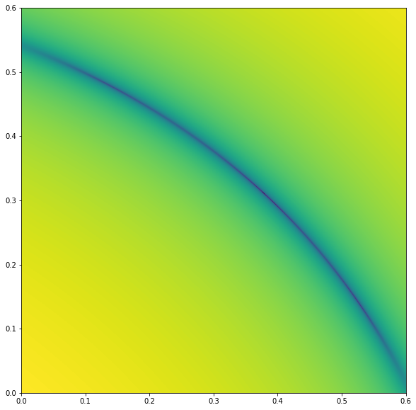
Looking at this heatmap, we immediately see two things. First, there is clearly a curved line through the parameter space where the error is lower than on either side. On closer examination, the exact curve is an axis-aligned hyperbola, and we’ll be able to characterize it soon. Second, along this curve, the story is more complicated. In fact, for this source curve there are three local minima.

But let’s take these in turn.

Signed area

Long story short, the main error-minimizing curve in the parameter space is the set of Béziers with the same signed area as the source curve. Mathematically, it is fairly easy to establish the connection between the two concepts: if the areas don’t match, it is impossible for the error norm to be small.

Here’s a visual demonstration of the importance of area. In a C-shaped curve, scaling both armlengths down or up affects the area directly, and it is clear that when the area is too small or too large, it cannot fit the source curve well.

Fortunately for us, it is especially easy to calculate and reason about area. Thanks to Green’s theorem, the equation for area of a curve tends to fairly simple, and with the normalization to the x-unit chord above, it actually becomes quite nice:

\[\mathrm{area} = \tfrac{3}{20}(2\delta_0 \sin \theta_0 + 2\delta_1 \sin \theta_1 - \delta_0 \delta_1 \sin(\theta_0 + \theta_1))\]

Immediately this formula buys us a lot; it’s quite straightforward to calculate $\delta_1$ given $\delta_0$.

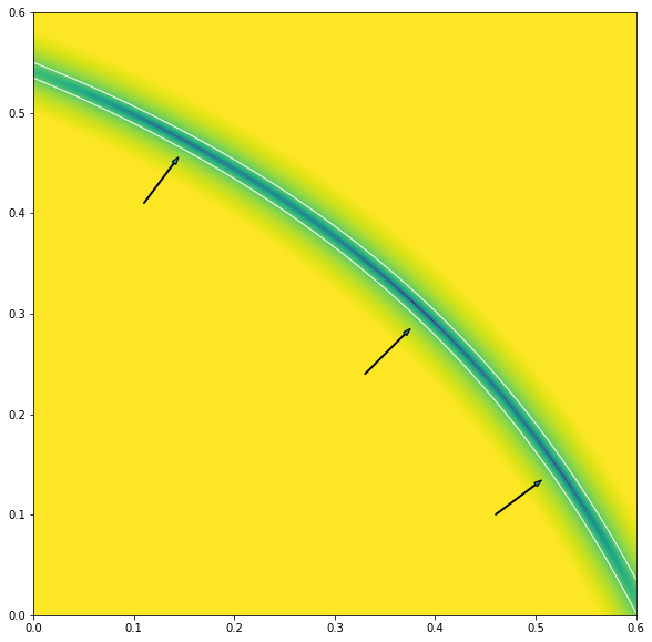
We can confirm visually that this equation for area predicts error; in the following graphic we’ve plotted lines for a small delta above and below the true value. The line of minimum error clearly follows the centerline. The graph also uses a colormap with enhanced contrast for low errors, which among other things more clearly displays the three local minima.

Circular arcs

In the case of fitting circular arcs, it’s already been shown by Spencer Mortenson that the standard approach of fitting the midpoint to lie on the circle doesn’t exactly minimize the error, though it’s pretty close. In this case, the optimal curve is symmetrical, so we can just set the arm lengths equal and solve the above equation (it becomes a simple quadratic). This approach is not significantly slower or more difficult than the usual.

The area of a circular arc with unit chord and a deflection of $\theta$ at each endpoint is:

\[\mathrm{area} = \frac{\frac{\theta}{\sin \theta} - \cos \theta}{4\sin \theta}\]

Applying the formula for area above, using the quadratic formula, and simplifying a bit, we get this value for the arm length:

\[\frac{2\sin \theta - \sqrt{4 \sin^2 \theta - \frac{20}{3}\sin(2\theta)\mathrm{area}}}{\sin(2\theta)}\]

The standard approach overshoots the radius everywhere except the endpoints and midpoint, so it will have an excess area. This approach undershoots at the midpoint and overshoots roughly at the one quarter and three quarter points, but with less absolute deviation. In any case, all approaches have $O(n^6)$ scaling, which is excellent. Only the constant factor varies, and only by a small amount. Mortenson’s approach minimizes the Fréchet distance, so in the end the choice boils down to which error metric we want to minimize.

Area has meaning

In addition to acting as a sensitive measure of overall curve-fit accuracy, area also has meaning of its own. In particular, when simplifying the outline of a glyph in a font, an area-preserving curve fit means that the amount of ink in a stroke is exactly preserved even if the shape is slightly distorted. As a font designer, I find that a desirable property.

Solving the second parameter

Restricting ourselves to area-preserving solutions means that we now have a one dimensional parameter space to search. Let’s plot the error from the above heatmap along the area-preserving curve, by plotting against $\delta_0$ and deriving $\delta_1$ from that:

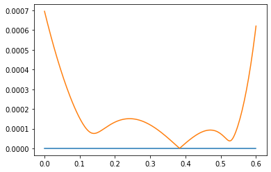
Here we can see the three local minima even more clearly. The cubic Béziers corresponding to each minimum are visually very similar, even though the arm lengths are quite different:

At this point, it would not be unreasonable to simply apply numerical techniques to find the minima, but we can do even better.

Ideally, we would like to find a measure of the curve that satisfies the following properties:

• It is a sensitive indicator of overall error.
• It takes the entire curve into account, not just local features.
• It is mathematically tractable.
• It is “most orthogonal” to the area measure.

Some candidates come close. For example, arc length (used in chapter 9 of my thesis) satisfies some of these, but in the case of a symmetric curve such as a circular arc is not orthogonal to area at all.

Again long story short, a winner is the first image moment, calculated in the direction of the chord from the start point to the end point, or we can say x-moment because with our chord normalization this is the $x$ axis. Generally, the first moment in 2D is computed in pairs, one for each direction, so it’s slightly odd that we’re only bothering with one and ignoring the other. But the requirement that it be as orthogonal as possible to area guides this choice.

It’s harder to visualize the difference in x-moment in a C-shaped curve, because the differences in the shapes of the curves are more subtle, but in a curve with more curvature variation, it’s clear enough. All these curves have the same area, but different values for x-moment:

Going back to the same-area slice through the error heatmap of our running example, plotting the x-moment makes it clear it accurately predicts error:

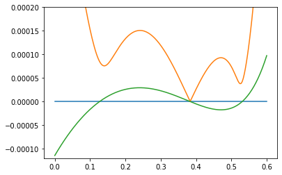
In particular, each of the three local minima of the error correspond closely to a zero-crossing of the x-moment. So now we just have to find the solutions of that equation.

Fortunately, Green’s theorem also helps us derive an efficient formula for computing the x-moment of our Bézier. It’s more fiddly, but the same basic idea as area:

\[\begin{align} \mathrm{moment_x} = \,\tfrac{1}{280}(\ &34 \delta_0 \sin \theta_0 \\ + \ & 50 \delta_1 \sin \theta_1 \\ + \ & 15 \delta_0^2 \sin \theta_0 \cos \theta_0 \\ - \ & 15 \delta_1^2 \sin \theta_1 \cos \theta_1 \\ - \ & \delta_0 \delta_1 (33\sin \theta_0 \cos \theta_1 + 9 \cos \theta_0 \sin \theta_1) \\ - \ &9 \delta_0^2 \delta_1 \sin(\theta_0 + \theta_1) \cos \theta_0 \\ + \ & 9 \delta_0 \delta_1^2 \sin(\theta_0 + \theta_1) \cos \theta_1 ) \end{align}\]

It’s perfectly reasonable to use numerical techniques to solve this equation (it’s much cheaper than computing an error norm relative to the original curve), but again, we can do better.

A quartic polynomial

We’re looking for the simultaneous solution of the area and x-moment constraints. Using some mathematical tricks (very similar to those used in the Penner paper), we can reduce the whole thing to a single quartic polynomial.

• Transform instances of $\delta_0 \delta_1$ into an equation of the form $a\delta_0 + b\delta_1 + c$.

• Replace all instances of $\delta_1$ by its area-preserving solution in terms of $\delta_0$.

• Multiply the polynomial by $(\delta_0 \sin (\theta_0 + \theta_1) - 2 \sin \theta_1)^2$.

Given a quartic polynomial, there are both analytical and numeric solutions (the latter can still be desirable because it can be tricky to achieve numerical robustness).

In addition to more efficient solving, the existence of a polynomial gives us great insight into the solution space, in particular the number of solutions.

The fourth solution

A quartic polynomial can have up to four solutions, but so far we’ve been talking about triplets of similar-shaped curves. What about the fourth?

It turns out that it’s also a valid solution of the area and x-moment constraints, but not at all close to the original curve, as it contains a loop. When computing signed area, the lobe enclosed by the loop has opposite sign as the rest of the curve, and similarly for moment. The area enclosed by the loop exactly balances out the excess area in the non-loop portion of the curve.

These two Béziers thus have the same signed area and x-moment, but are clearly not similar:

Thus, in the general case we can talk about a triplet of similar curves and one “nemesis” that has a different loop structure, all of which share the same area and x-moment.

Depending on the application, it may be worth considering all four solutions. In particular, if the source curve has such a loop (or a cusp), it’s desirable to find the Bézier that fits it most closely. But in the case where source curve has no such loop, solutions with such extreme values for arm length can be immediately excluded. A reasonable goal of a curve fitting algorithm is that if you put a cubic Bézier in as the source curve, you should get exactly the same Bézier out, and that can include curves with loops and cusps. Many approaches in the literature do not have this property.

Near misses

If we only consider exact solutions of the x-moment constraint, we may miss some error minima. Consider the Euler spiral with deflections of 0.285 and 0.35 radians as a source curve to fit. The graph of x-moment and error looks like this:

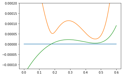
Here, on the right side of the graph, the x-moment approaches zero but doesn’t actually cross the axis. Even so, the error there is lower than the actual crossing of the axis on the left. Fortunately, it is not too hard to take these into account as well, just consider places where the derivative of the x-moment is zero in addition.

The Penner paper described a “surprising oval” of solutions found by the Orthogonal Distance Fitting approach but missed by the solver based on center of mass. These are the same “near misses,” and taking them into account ensures that the error is continuous with respect to small changes in the source curve, even when the solution jumps from one branch to another.

Conclusion and discussion

We have presented a highly efficient and accurate solution to cubic Bézier curve fitting, along with some insight into the nature of cubic Béziers which make such a solution tricky. The solution is determined from direct solving of a polynomial rather than iterative optimization. In cases where there are multiple local minima, it reliably finds all of them and lets us pick the global optimum.

Because of branches and double roots in this polynomial, the parameters of the solution can move around a lot or even jump in response to small changes in the source curve. It is the nature of cubic Béziers to be able to fit a source curve very accurately (with $O(n^6)$ scaling), but if these optimized curves are to be used as masters in an interpolation scheme, for example for variable fonts, they are not necessarily interpolation compatible, meaning that the result of interpolating between two of these masters may not closely resemble either one of them.

Thanks to Bernat Guillen for discussion. Discuss on Hacker News and TypeDrawers.