Cleaner parallel curves with Euler spirals

Determining parallel curves is one of the basic 2D geometry operations. It has obvious applications in graphics, being the basis of creating a stroke outline from a path, but also in computer aided manufacturing (determining the path of a milling tool with finite radius) and path planning for robotics. There are plenty of solutions in the literature by now, but in this post I propose a cleaner solution.

A good survey paper is Comparing Offset Curve Approximation Methods. The main difference between these approaches is the choice of curve representation. An example of a curve representation highly specialized for deriving parallel curves is the Pythagorean Hodograph. This parallel curve of a Pythagorean Hodograph is an exact parametric polynomial curve, but approximation techniques are still needed in practice, both to convert the source curve into the representation, and because the resulting curves are higher order rational polynomials, which require further approximation to convert into, say, cubic Béziers.

Specifically, this blog proposes piecewise Euler spirals as a curve representation particularly well suited to the parallel curve problem.

There’s an implementation of many of these ideas (currently still in PR stage) in kurbo. I also used a colab notebook to explore a bunch of the math, and I’ve made a copy of that available as well.

The cusp

One of the things that makes parallel curves special is that cusps often appear. In particular, a cusp appears whenever the radius of curvature of the source curve matches the offset. This is classified as an ordinary cusp and is a feature of many curve families – we’ll quantify that a bit more below.

A common feature of algorithms for computing parallel curves is identifying the location of the cusp, and subdividing there. That basically means solving for the specific value of curvature (the reciprocal of the offset distance). If the source curve is a cubic Bézier, there can be up to four such cusps, and finding them requires some nontrivial numerical solving.

Curvature as a function of arclength

A theme of my approach to parallel curves (and much of my curve work in general, including my thesis), is to consider the relationship of curvature to arclength. A concrete intuition is that it is the position of the steering wheel as a car drives along the curve at constant speed. For some curves, curvature can be represented as a closed-form analytical formula as a function of arclength (the Cesàro equation), but in general determining the relation requires numerical techniques. For example, in the Euler explorer, there’s a plot of curvature as a function of arclength below the interactive cubic Bézier. Experimenting with that is an excellent way to develop intuition.

One curve that does have an especially simple Cesàro equation is the Euler spiral. An Euler spiral segment has this formula:

\[\kappa(s) = \kappa_0 + \kappa_1 s\]

(A note for those trying to follow along with the detailed math and code: most of the math and numerical code uses $-0.5 \leq s \leq 0.5$ because it helps exploit even/odd symmetries, but the convention for parametrized curves, including the ParamCurve trait in kurbo, is $0 \leq s \leq 1$. Thus, you’ll frequently see offsets of 0.5. Similarly, you’ll see various scaling to the actual arc length, while the parametrized curve convention assumes an arc length of 1. In this blog, we’ll skim over such details, as the goal is to provide intuition without too much clutter from details.)

The parallel curve of an Euler spiral

In general, most curves do not have a simple formula for their parallel curve. The obvious exception is a circular arc, for which the parallel curve is another circular arc. Another curve family with tractable representation for its parallel curve is Pythagorean Hodographs.

Thanks to its exceptionally simple formulation as a Cesàro equation, the Euler spiral is one of the rare curves with a simple closed-form equation for its parallel curve. That equation was first published in a 1906 paper by Heinrich Wieleitner, Die Parallelkurve der Klothoide. For those who don’t read German, Rahix has kindly provided a translation into English: PDF, TeX source.

Going over this math, I see Wieleitner missed an opportunity for further simplification. The style at the time was to write the Cesàro equation in terms of the radius of curvature (the reciprocal of curvature), but especially for the Euler spiral and its parallel curve, using curvature directly yields a much simpler equation. With the cusp located at $s_0$, the equation is gratifyingly simple:

\[\kappa(s) = \frac{c}{\sqrt{s - s_0}} + \frac{1}{l}\]

The equation is graphed below, and clicking on it links to a Desmos calculator graph with sliders for the parameters.

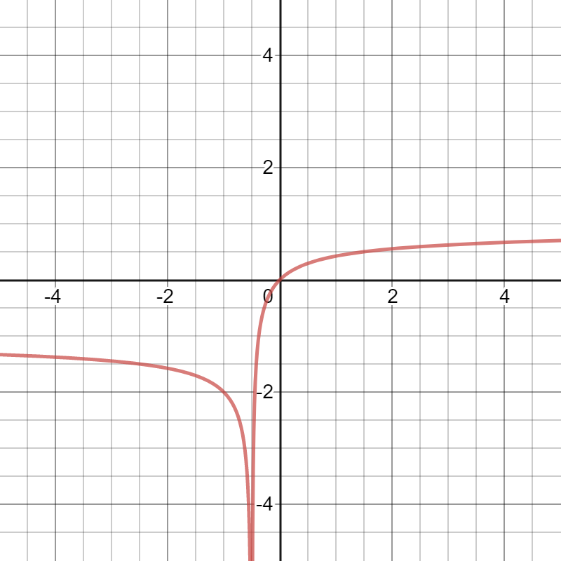
Here $c$ is a coefficient dependent on the parameters of the spiral. To connect it to the notation in the Wieleitner paper, $c = a / \sqrt{2 l^3}$, and $s_0 = -a^2/{2l}$. I’ve also made a Desmos calculator graph that interactively demonstrates the equivalence of this equation and the more involved one from the Wieleitner paper.

There are a number of other curves that have a cusp similar to the above, with characteristic inverse-square root curvature. The clearest connection is the circle involute, which is the same but without the $1/l$ term, or in other words the Euler spiral parallel curve approaches the circle involute as the offset goes to infinity. This provides intuition for the fact that a circle involute is its own parallel curve. The circle involute is perhaps most famous as the optimized profile for meshing gear teeth, transferring force smoothly with no slop or friction.

Other curves with a similar cusp include the cycloid (as well as its many variants including epicycloid, hypocycloid, astroid, deltoid, cardioid, and nephroid), as well as the semicubical parabola. The latter is of particular interest because it can be exactly represented as a case of a cubic Bézier (it is when the control arms form a symmetrical X).

The parallel curve of the Euler spiral is perfectly cromulent, and, following the tradition of Pythagorean Hodograph curves and their higher-order rational polynomials, we could simply require everything downstream to simply deal with them. But to make that downstream processing easier, we will convert back to piecewise Euler spirals, a more tractable representation.

Geometric Hermite interpolation

Hermite interpolation is a well known technique. In its simplest form, it is used to generate a piecewise polynomial approximation to some function, where the parameters for each polynomial segment are determined from the values and derivatives of the endpoints. For example, in cubic Hermite interpolation, a cubic polynomial is determined from the values and first derivatives at the endpoints – four values, corresponding to four coefficients for the polynomial. The result is C1 continuous as the derivatives exactly match (and are equal to the source curve).

In 2D, there is a distinction between C1 and G1 (geometric) continuity. In C1 continuity, the full derivatives must match, both direction and magnitude. For applications such as animating motion curves, the magnitude is important (it represents speed of motion), but for curves, it is not. G1 continuity requires that the tangents match, but does not specify the magnitude of the derivatives.

In these applications, geometric Hermite interpolation is more efficient, as all parameters of the curve are available to make the shape fit. The Euler spiral is especially well suited to geometric Hermite interpolation, and there is literature on this topic. For reasonable assumptions of smoothness (excluding fractal curves but including simple cusps), the accuracy scales as $O(n^4)$ – a doubling of the number of subdivisions reduces the error by a factor of 16. This scaling is the same as cubic Hermite interpolation of a 1D function, not surprising as an Euler spiral segment approximates a cubic polynomial when $y$ values are small.

Section 8.2 of my thesis provides a secant method for determining the Euler spiral parameters from the G1 Hermite constraints, and that’s implemented in the fit_euler method in the kurbo PR. That’s a good technique and its convergence is excellent (quadratic, as typical for Newton-style solvers for near-linear problems), but I’ve also been experimenting with ways to do it better. The linked notebook explores a polynomial approximation (based on 2D Taylor’s series) that is much faster – 7ns vs 240ns in my measurements, and should be very accurate over a wide range of parameters. I’m not quite done making the error bounds rigorous, but this approach should help make the overall algorithm lightning-fast.

Geometric Hermite interpolation works well to approximate the parallel curve of an Euler spiral segment with another Euler spiral segment:

The true parallel curve is in blue, and the approximation in red. It has the same rough shape, but bulges out in the middle. We need to be able to estimate that error in order to make a more accurate approximation.

A simple, accurate error metric

The most common approach to approximation given a target error bound is adaptive subdivision: approximate the error, and if it exceeds the target, subdivide. Evaluating the error is not always easy; most generally, it’s based on numerical techniques such as evaluating the curve at several points along its length and testing how near those points lie to the source curve.

Fortunately, for approximating an Euler spiral parallel curve using an Euler spiral, there is an extremely simple formula for the error. In fact, it’s possible to avoid the adaptive subdivision altogether, and precisely predict how many subdivisions are needed to meet an error bound, as well as analytically place the subdivisions so each segment has the same error.

Normalized to a chord length of 1, where the arc length of the Euler spiral segment is $a$, the error for approximating an Euler spiral segment with central curvature $\kappa_0$ and curvature variation $\kappa_1$ offset by distance $l$ is:

\[E \approx 0.005a\left|\frac{1}{\kappa_0 a^{-1} + l^{-1}}\right|\kappa_1 ^ 2\]

The $\kappa_0 a^{-1} + l^{-1}$ term represents a distance from the cusp; the error scales in inverse proportion to this distance. Also note that $\kappa_1$ scales as the square of the number of subdivisions, so the entire formula scales as the fourth power, as expected.

Precise subdivision

Given such a simple formula for the error metric, we can do better than the usual adaptive subdivision approach, which simply evaluates the error metric and subdivides in half if the threshold is not met. We can compute exactly how many subdivisions are needed, and where to split so the error of each subdivided segment is the same.

More details are in the attached notebook, but the essence is this. If $s_i$ is chosen on the original curve according to the following formula, then error of each segment $s_i$ to $s_{i + 1}$ will be close to equal:

\[s_i = s_0 + (t_0 + i \Delta t)^\frac{4}{3}\]

Here $s_0$ is the location of the cusp. The key to using this formula is to choose $t_0$ so $s_0$ lands on one of the endpoints, then $\Delta t$ and $n$ so that $t_0 + n \Delta t$ lands on the other, and $n$ is the minimum value that still meets the error bound. The details are a bit fiddly, though not expensive to compute, and can be found in the notebook.

I should note in fairness that this doesn’t result in exactly equal error, but slightly undershoots for segments very close to the cusp. The resulting inefficiency is probably a few percent in practice, in my opinion well worth having such a direct solution.

The above image shows the subdivisions produced by this precise approach, to an accuracy of about a tenth of a pixel, quite adequate for font and 2D artwork applications. Generally there are two to four subdivisions when there’s no cusp, and up to twice that when the cusp is present. The lead image of this blog has an accuracy of 10^-5 pixel, which should be more than adequate for just about any application, and the number of segments is still quite manageable. I like the image because it shows how the number of subdivisions smoothly increases near the cusps.

Euler spiral or parabola

At heart, the algorithm is similar to the subdivision into parabolas. Why Euler spirals instead?

A particularly tricky case for a parallel curve algorithm is when the input curve is a circular arc with curvature nearly matching the offset distance. The exact result is another circular arc with very small radius. However, using Béziers as the curve representation means that the curvature will “ripple” due to approximation errors. In the worst case, these ripples straddle the critical curvature value for generating cusps. Each quadratic Bézier can generate two such cusps. The finer the subdivision (for more accuracy in the result), the more cusps!

Of course, a circular arc is a case the Euler spiral can represent exactly, and its parallel curve also has zero error.

To summarize, approximating a curve by Béziers can add cusps to the corresponding parallel curve, while approximating a curve by Euler spirals can remove them without sacrificing accuracy. This observation is the main reason I claim that Euler spirals are a “cleaner” solution to the parallel curve problem.

Euler spirals to cubic Béziers

A previous blog post, Secrets of smooth Béziers revealed, addressed the question of fitting a cubic Bézier to approximate an Euler spiral segment. There is more to be said on the topic, but here I will show a simple and appealing solution.

Graphic designers using cubic Béziers are commonly taught that smooth curves result when the distance from the control point to the endpoint is approximately 1/3 the distance between the endpoints. A more precise refinement of this concept is to draw a parabola around each endpoint, with the vertex 1/3 way along the chord, and a distance of 2/3 in the orthogonal direction. The Euler spiral approximation is simply the point along that parabola in the desired tangent direction.

In the symmetrical case, this solution is equivalent to the standard solution for approximating a circular arc using a cubic Bézier, as can be seen with a bit of trigonometry. What’s less obvious is that it remains very good even in the non-symmetrical case, in particular the arclength of the Bézier matches the true curve pretty well. The error scaling is as the fifth power, which is better than fourth power scaling of using standard Hermite interpolation (it consistently undershoots arclength), but not as good as the sixth power scaling that is theoretically possible, as shown in High Accuracy Geometric Hermite Interpolation. However, actually achieving that requires some difficult numerical techniques, as compared with the simple parabola rule stated above.

The error bound, as well as the tightness of its analytical estimation, can be visualized in this image:

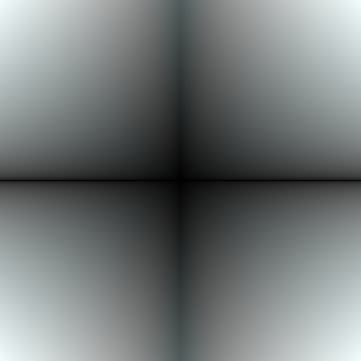
Here, k0 is the horizontal axis and k1 is the vertical. The horizontal axis (k1 = 0) represents perfect circular arcs, while the vertical (k0 = 0) is “s” curves with odd symmetry; both cases have particularly low error. Black represents zero error, red the true error, and cyan the approximate error (see the fit_cubic_plot function in the examples in the associated kurbo PR for the error bound and the code used to plot the above). Thus, neutral gray means that the error bound is tight.

This simple fitting with $n^5$ scaling, is appealing because it is very fast to evaluate, and in most cases will produce cubic Béziers with a comfortable but not excessive safety margin for accuracy, especially since earlier stages of the approximation pipeline scale as $n^4$.

Conclusion

The parallel curve problem has a well deserved reputation for being tricky. However, a large part of the problem is the choice of Béziers as the underlying curve representation – the parallel curve of a Bézier is a difficult beast to analyze and approximate, prone to cusps in hard-to-predict locations. By contrast, an Euler spiral representation of the source curve simplifies these problems, with a clean analytical solution for its parallel curve.

In demonstrating the advantages of an Euler spiral representation, this blog post has presented a number of new results:

• A very simple closed form Cesàro equation for the Euler spiral parallel curve, relating it to the involute of a circle.

• A simple analytical error metric for approximating this parallel curve as piecewise Euler spirals.

• An extremely efficient algorithm for geometric Hermite interpolation of Euler spirals.

• An efficient and direct approximation of Euler spirals into cubic Béziers, also with tight error bounds.

The more I work with Euler spirals, the more I find them to be a simple, efficient, and tractable representation of curves. For example, because they’re defined using an arc length parameter, inverse arc length problems are nearly trivial. To look at the literature, working with Euler spirals would seem to require solutions to tricky problems such as evaluating Fresnel integrals, but in practice, highly efficient polynomial approximations work well, producing results of arbitrarily high precision with a modest (and predictable!) increase in the number of subdivisions. I’ve demonstrated how this curve representation is especially well suited to determining parallel curves, and also look forward to exploring its suitability for other classical 2D geometry problems.

The actual implementation of the parallel curve in the kurbo PR is less than 100 lines of code, including handling of the cusps and careful error bounds. I think that provides further support for the claim that Euler spirals support a “cleaner” implementation than other curve representations. I haven’t done careful benchmarking of the end-to-end implementation yet, but expect it to be very fast, certainly based on performance of the important primitives. Speed is important to me, as I want these operations available in design applications, providing accurate and powerful geometry operations with smooth interactivity. That’s a major reason I’m choosing Rust for the implementation.

Lastly: the results in this blog post are determined mostly through experimentation, and validated through testing (randomized in many cases). If it were an academic paper, it would derive error bounds and related results rigorously using mathematical techniques. If that sounds fun, get in touch and let’s discuss collaborating on a paper.

Discuss on Hacker News.