Simplifying Bézier paths
Finding the optimal Bézier path to fit some source curve is, surprisingly, not yet a completely solved problem. Previous posts have given good solutions for specific instances: Fitting cubic Bézier curves primarily addressed Euler spirals (which are very smooth), while Parallel curves of cubic Béziers rendered parallel curves. In this post, I describe refinements of the ideas to solve the much more general problem of simplifying arbitrary paths. Along with the theoretical ideas, a reasonably solid implementation is landing in kurbo, a Rust library for 2D shapes.
The techniques in this post, and code in kurbo, come close to producing the globally optimum Bézier path to approximate the source curve, with fairly decent performance (as well as a faster option that’s not always minimal in the number of segments), though as we’ll see, there is considerable subtlety to what “optimum” means. Potential applications are many:
- Simplification of Bézier paths for more efficient publishing or editing
- Conversion of fonts into cubic outlines
- Tracing of bitmap images into vectors
- Rendering of offset curves
- Conversion from other curve types including NURBS, piecewise spiral
- Distortions and transforms including perspective transform
While the primary motivation is simplification of an existing Bézier path into a new one with fewer segments, the techniques are quite general. One of the innovations is the ParamCurveFit trait, which designed for efficient evaluation of any smooth curve segment for curve fitting. Implementations of this trait are provided for parallel curves and path simplification, but it is intentionally open ended and can be implemented by user code.
This work is an opportunity to revisit some of the topics from my thesis, where I also explored systematic search for optimal Bézier fits. The new work is several orders of magnitude faster and more systematic about not getting stuck in local minima.
The ParamCurveFit trait
At its best, a trait in Rust is a way to model some fact about the problem, then serves as an interface or abstraction boundary between pieces of code. The ParamCurveFit trait models an arbitrary curve for the purpose of generating a Bézier path approximating that source curve. The key insight is to sample both the position and derivative of the source curve for given parameters, and there is also a mechanism for detecting cusps (particularly important for parallel curves).
The curve fitting process uses those position and derivative samples to compute candidate approximation curves, then measure the error between source curve and approximation.
Two implementations are provided: parallel curves of cubic Béziers, and arbitrary Bézier paths for simplification. Implementing the trait is not very difficult, so it should be possible to add more source curves and transformations, taking advantage of powerful, general mechanisms to compute an optimized Bézier path.
The core cubic Bézier fitting algorithm is based on measuring the area and moment of the source curve. A default implementation is provided by the ParamCurveFit trait implementing numerical integration based on derivatives (Green’s theorem), but if there’s a better way to compute area and moment, source curves can provide their own implementation.
For Bézier paths, an efficient analytic implementation is possible. No blog post of mine is complete without some reference to a monoid, and this one does not disappoint. It’s relatively straightforward to compute area and moments from a cubic Bézier using symbolic evaluation of Green’s theorem. The area and moments of a sequence of Bézier segments is the sum of the individual values for each segment. Thus, we precompute the prefix sum of the areas and moments for all segments in a path, then can query an arbitrary range in O(1) time by taking the difference between the end point and the start point.
Error metrics
The problem of finding an optimal Bézier path approximation is always relative to some error metric. In general, an optimal path is one with a minimal number of segments while still meeting the error bound, and a minimal error compared to other paths with the same number of segments. A curve fitting algorithm will evaluate many error metrics, at least one for each candidate approximation to determine whether it meets the error bound. The simplest technique subdivides in half when the bound is not met, but a more sophisticated approach attempts to optimize the positions of the subdivision points as well.
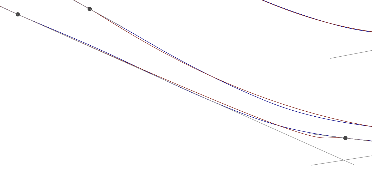
The main error metric used for curve fitting is Fréchet distance. Intuitively, it captures the idea of the maximum distance between two curves while also preserving orientation of direction along a path (the related Hausdorff metric does not preserve orientation and so a curve with a sharp zigzag may have a small Hausdorff metric measured against a straight line). The difference is shown in the following illustration:

Computing the exact Fréchet distance between two curves is not in general tractable, so we have to use approximations. It is important for the approximation to not underestimate, as this will yield a result that exceeds the error bound.
The classic Tiller and Hanson paper on parallel curves proposed a practical, reasonably accurate, and efficient error metric to approximate Fréchet distance. It samples the source curve at n points, and for each point casts a ray along the normal from the point, detecting intersections with the cubic approximation. The maxium distance from a source curve point to the corresponding intersection is the metric.
Unfortunately, there is a case Tiller-Hanson handles poorly, and equally unfortunately, it does come up when doing simplification of arbitrary paths. Consider a superellipse shape, approximated (badly) by a cubic Bézier with a loop. The rays strike only parts of the approximating curve and miss the loop entirely.

Increasing the sampling density helps a little but doesn’t guarantee that the approximation will be well covered. Indeed, it is the high curvature in the source curve that makes this coverage more uneven.
A more robust metric is to parametrize the curves by arc length, and measure the distance between samples that share a corresponding portion of the total arc length. This ensures that all parts of both curves are considered. When curves are close (which is a valid assumption for curve fitting), it closely approximates Fréchet distance, though potentially can overestimate (because nearest points don’t necessarily coincide with arc length parametrization) and underestimate due to sampling.

However, arc length parametrization is considerably slower (about a factor of 10) because it requires inverse arc length computations. The approach implemented in kurbo#269 is to classify whether the source curve is “spicy” (considering the deltas between successive normal angles) and use the more robust computation only in those cases.
Finding subdivision points
An extremely common approach is adaptive subdivision. Compute an approximation, evaluate the error metric, and subdivide in half when it is exceeded. This approach is simple, robust, and performant (the total number of evaluations is within a factor of 2 of the number of segments). However, it tends to produce results with more segments than absolutely needed. In the limit, it tends to be about 1.5 times the optimum.
Fancier techniques try to optimize the subdivision points to reduce the number of segments. That is equivalent to dividing the source curve into ranges such that each range is just barely below the threshold; ironically, it basically amounts to maximizing the error metric right up to the constraint.
One technique is given in section 9.6.4 of my thesis. Basically you start on one end and for each segment find a subdivision point from the last point to one that’s just barely under the error threshold. Under the assumption that errors are monotonic (which is not always going to be the case), this finds the global minimum number of segments needed. The last segment will have an error well below the threshold. Then, another search finds the minimum error for which this process yields the same number of segments. Again, if error is monotonic, the result is the Fréchet distance of all segments being equal, which is (at least roughly) equivalent to the overall Fréchet distance being minimized.
For smooth source curves, monotonic error is a reasonable assumption. Even so, the above technique seems to work fairly robustly, producing fewer segments than simple adaptive subdivision, though it is somewhere around 50x slower.
There may be scope to improve this optimization process further. Crates like argmin implement general purpose multidimensional optimization algorithms, and it’s worth exploring whether those could produce equally good results with fewer evaluations.
Bumps
Something unexpected arose during testing: the resulting “optimum” simplified paths had bumps. Obviously at first I thought this was some kind of failure of the algorithm, but now I think something more subtle is happening.
The solution below is with an error tolerance of 0.15, which produces a total of 43 segments:

Near the bottom is a bump. It almost looks like a discontinuity (and other similar examples even more so), but on closer examination it is simply one very long and one very short control arm (ie distance between control point and corresponding endpoint), which creates a high degree of curvature variation:
The underlying problem is that Fréchet distance optimizes only for a distance metric, and does not by itself guarantee a low angle (or curvature) error. In many cases, these objectives are not in tension – the curve that minimizes distance error also smoothly hugs the source curve. But there are cases where there is in fact a tradeoff, and when such tradeoffs exist, agressively optimizing for one causes the other to suffer.
For this particular range of the test data, I believe the Fréchet-minimizing cubic Bézier approximation does indeed exhibit the bump; tweaking the parameters will certainly improve smoothness, but also result in a greater distance from the source curve.
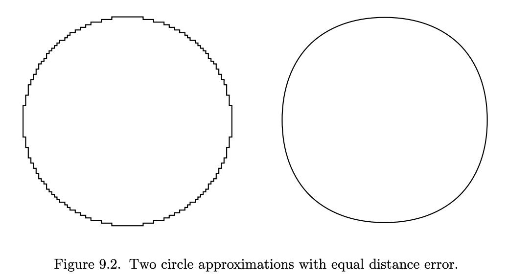
This state of affairs is not acceptable in most applications. It is evidence that Fréchet does not capture all aspects of the objective function. Section 9.2 of the thesis discusses this point.
Given that aggressively optimizing Fréchet may give undesirable results, what is to be done? The most systematic approach would be to design an error metric that takes both distance and angle into account, and calibrate it to correlate strongly with perception. That is perhaps a tall order, requiring research to properly establish tuning parameters, and likely with complexity and runtime performance implications to evaluate. Even so, I think it should be pursued.
A simpler approach, implemented in the current code, is to recognize that these bumpy cubic Béziers can be recognized by their parameters; when the distance from the endpoints to the control points roughly equal to the chord length, then curves can have cusps or nearly so. These are the δ values from the core quartic-based curve fitting solver; a simple approach would be to simply exclude curves with δ values greater than some threshold (0.85 works well), and this also improves performance by decreasing the number of error evaluations needed, but a more sophisticated approach is to multiply the error by a penalty factor for larger δ. One advantage of the latter approach is that it is still possible to fit every actual exact Bézier input.
Applying this tweak gives a much smoother result, though it does require one more segment (44 rather than 43 previously).

Another point to make at this point is that the number of path segments needed scales very gently as the error bound is tightened; changing the threshold from 0.15 to 0.05 increases the number of segments only from 44 to 60. In the limit, the error scales as O(n^6). This extremely fast convergence is one reason that cubic Béziers can be considered a universal representation of curved paths; while some other representation such as NURBS may be able to represent conic sections exactly, any such smooth curve can be approximated to an extremely tight tolerance using a modest number of cubic segments. The path simplification technique in this blog (and in kurbo) gives a practical way to actually attain this degree of accuracy.

And taking the error down to 0.01 requires only 90 segments. This creates an extremely close fit to the source curve, still without requiring an excessive number of segments.

These are vector images, so please feel free to open them in a new tab and zoom in to inspect them more carefully. You should see all solutions display an impressive amount of control over the curvature variation afforded by cubic Béziers. The code is available, so also feel free to experiment with it with your own test data and for your own applications. I’m especially interested in cases where the algorithm doesn’t perform well; it hasn’t been carefully validated yet.
Low pass filtering
The “best” curve depends on the use case. When the source curve is an authoritative source of truth, then making each segment G1 continuous with it at the endpoints is reasonable. However, when the source curve is noisy, perhaps because it’s derived from a scanned image or digitizer samples, then an optimum simplified path may have angle deviations relative to the source that make the overall curve smoother.
I haven’t been working from noisy data and haven’t done experiments, but I do suggest a possibility: use a global optimizing technique such as that provided by argmin, and jointly optimize both the location of the subdivision points and a delta to be applied to the angle (equally on both sides of a subdivision, so the resulting curve remains G1). Another possibility is to explicitly apply a low-pass filter, tuned so the amount of smoothing is consistent with the amount of simplification. In any case, using the existing code with no further tuning may yield less than optimum results.
Discussion
The current code in kurbo is likely considerably better than what’s in your current drawing tool, but curve fitting remains work in progress. The core primitive feels solid, but applying it might require different tuning depending on the specifics of the use case. I invite collaboration along these lines.
Many of the points in this blog were discussed in Zulip threads, particularly curve offsets and More thoughts on cubic fitting. The Zulip is a great place to discuss these ideas, and we welcome newcomers and people bringing questions.
Thanks to Siqi Wang for insightful questions and making test data available.