A sort-middle architecture for 2D graphics
In my recent piet-gpu update, I wrote that I was not satisfied with performance and teased a new approach. I’m on a quest to systematically figure out how to get top-notch performance, and this is a report of one station I’m passing through.
To recap, piet-gpu is a new high performance 2D rendering engine, currently a research protoype. While most 2D renderers fit the vector primitives into a GPU’s rasterization pipeline, the brief for piet-gpu is to fully explore what’s possible using the compute capabilities of modern GPUs. In short, it’s a software renderer that is written to run efficiently on a highly parallel computer. Software rendering has been gaining more attention even for complex 3D scenes, as the traditional triangle-centric pipeline is less and less of a fit for high-end rendering. As a striking example, the new Unreal 5 engine relies heavily on compute shaders for software rasterization.
The new architecture for piet-gpu draws heavily from the 2011 paper High-Performance Software Rasterization on GPUs by Laine and Karras. That paper describes an all-compute rendering pipeline for the traditional 3D triangle workload. The architecture calls for sorting in the middle of the pipeline, so that in the early stage of the pipeline, triangles can be processed in arbitrary order to maximally exploit parallelism, but the output render still correctly applies the triangles in order. In 3D rendering, you can almost get away with unsorted rendering, relying on Z-buffering to decide a winning fragment, but that would result in “Z-fighting” artifacts and also cause problems for semitransparent fragments.
The original piet-metal architecture tried to avoid an explicit sorting step by traversing the scene graph from the root, each time. The simplicity is appealing, but it also required redundant work and limited the parallelism that could be exploited. The new architecture adopts a similar pipeline structure as the Laine and Karras paper, but with 2D graphics “elements” in place of triangles.
Central to the new piet-gpu architecture, the scene is represented as a contiguous sequence of these elements, each of which has a fixed-size representation. The current elements are “concatenate affine transform”, “set line width”, “line segment for stroke”, “stroke previous line segments”, “line segment for fill”, and “fill previous line segments”, with of course many more elements planned as the capability of the renderer grows.
While triangles are more or less independent of each other aside from the order of blending the rasterized fragments, these 2D graphics elements are a different beast: they affect graphics state, which is traditionally the enemy of parallelism. Filled outlines present another challenge: the effects are non-local, as the interior of a filled shape depends on the winding number as influenced by segments of the outline that may be very far away. It is not obvious how a pipeline designed for more or less independent triangles can be adapted to such a stateful model. This post will explain how it’s done.
Scan
In general, a sequence of operations, each of which manipulates state in some way, must be evaluated sequentially. An extreme example is a cryptographic hash such as SHA-256. A parallel approach to evaluating such a function would upend our understanding of computation.
However, in certain cases parallel evaluation is quite practical, in particular when the change to state can be modeled as an associative operation. The simplest nontrivial example is counting; just divide up the input into partitions, count each partition, then sum those.
Can we design an associative operation to model the state changes made by the elements of our scene representation? Almost, and as we’ll see, it’s close enough.
At this stage in the pipeline, there are three components to our state: the stroke width, the current affine transform, and the bounding box. Written as sequential pseudocode, our desired state manipulation looks like this:
Input an element.
If the previous element was "fill" or "stroke", reset the bounding box.
If the element is:
    "set line width", set the line width to that value.
    "concatenate transform", set the transform to the current transform times that.
    "line segment for fill," compute bounding box, and accumulate.
    "line segment for stroke," compute bounding box, expand by line width, and accumulate.
    "fill", output accumulated bounding box
    "stroke", output accumulated bounding box
Note that most graphics APIs have a “save” operation that pushes a state onto a stack, and “restore” to pop it. Because we desire our state to be fixed-size, we’ll avoid those. Instead, to simulate a “restore” operation, if the transform was changed since the previous “save,” the CPU encodes the inverse transform (this requires that transforms be non-degenerate, but this seems like a reasonable restriction).
As the result of such processing, each element in the input is annotated with a bounding box, which will be used in later pipeline stages for binning. The bounding box of a line segment is just that segment (expanded by line width in the case of strokes), but for a stroke or fill it is the union of the segments preceding it.
Given the relatively simple nature of the state modifications, we can design an “almost monoid” with an almost associative binary operator. I won’t give the whole structure here (it’s in the code as [element.comp]), but will sketch the highlights.
When modeling such state manipulations, it helps to think of the state changes performed by some contiguous slice of the input, then the combination of the effects of two contiguous slices. For example, either or both slices can set the line width. If the second slice does, then at the end the line width is that value, no matter what the first slice did. If it doesn’t, then the overall effect is the same as the first slice.
The effect on the transform is even simpler, it’s just multiplication of the affine transforms, already well known to be associative (but not commutative).
Where things get slightly trickier is the accumulation of the bounding boxes. The union of bounding boxes is an associative (and commutative) operator, but we also need a couple of flags to track whether the bounding box is reset. However, in general, affine transformations and bounding boxes don’t distribute perfectly; the bounding box resulting from that affine transformation of a bounding box might be larger than the bounding box of transforming the individual elements.

For our purposes, it’s ok for the bounding box to be conservative, as it’s used only for binning. If we restricted transforms to axis-aligned, or if we used a convex hull rather than bounding rectangle, then transforms would distribute perfectly and we’d have a true monoid. But close enough.
When I wrote my prefix sum blog post, I had some idea it might be useful in 2D, but did not know at that time how central it would be. Happily, that implementation could be adapted to handle the transform and bounding box calculation with only minor changes, and it’s lightning fast, as we’ll see below in the performance discussion.
Note that the previous version of piet-gpu (and piet-metal before it) required the CPU to compute the bounding box for each “item.” Part of the theme of the new work is to offload as much as possible to the GPU, including bounding box
Binning
While element processing is totally different than triangle processing in the Laine and Karras paper, binning is basically the same. The purpose of binning is fairly straightforward: divide the render target surface area into “bins” (256x256 pixels in this implementation), and for each bin output a list of elements that touch the bin, based on the bounding boxes as determined above.
If you look at the code, you’ll see a bunch of concern about right_edge, which is in service of the backdrop calculation, which we’ll cover in more detail below.
The binning stage is generally similar to cudaraster, though I did refine it. Where cudaraster launches a fixed number of workgroups (designed to match the number of Streaming Multiprocessors in the hardware) and outputs a linked list of segments, one per workgroup and partition, I found that this created a significant overhead in the subsequent merge step. Thus, my design outputs a contiguous segment per bin and partition, which allows for more parallel reading in the merge step, though it has a small overhead of potentially outputting empty segments (I suspect this is the reason Laine and Karras did not pursue the approach). In both cases, the workgroups do not need to synchronize with each other, and the elements within an output segment are kept sorted, which reduces the burden in the subsequent merge step.
The binning stage is also quite fast, not contributing significantly to the total render time.
Why such large bins, or, in other words, so few of them? If binning is so fast, it might be appealing to bin all the way down to individual tiles. But the design calls for one bin per thread, so that would exceed the size of a workgroup (workgroup size is generally bounded around 1024 threads, and very large workgroups can have other performance issues). Of course, it may well still be possible to improve performance by tuning such factors; in general I used round numbers.
Coarse rasterization
This pipeline stage was by far the most challenging to implement, both because of the grueling performance requirements and because of how much logic it needed to incorporate.
The core of the coarse rasterizer is very similar to cudaraster. Internally it works in stages, each cycle consuming 256 elements from the bin until all elements in the bin have been processed.
-
The first stage merges the bin outputs, restoring the elements to sorted order. This stage repeatedly reads chunks generated in the binning stage until 256 elements are read (or the end of the input is reached).
-
Next is the input stage, with each thread reading one element. It also compute the coverage of that element, effectively painting a 16x16 bitmap. There’s special handling of backdrops as well, see below.
-
The total number of line segments is counted, and space in the output is allocated using an atomic add.
-
As in cudaraster, segments are output in a highly parallel scheme, with all output segments evenly divided between threads, so each thread has to do a small stage to find its work item.
-
The commands for a tile are then written sequentially, one tile per thread. This lets us keep track of per-tile state, and there tend to be many fewer commands than segments.
This is called “coarse rasterization” because it is sensitive to the geometry of path segments. In particular, coverage of tiles by line segments is done with a “fat line rasterization” algorithm:

Backdrop
A special feature of coarse rasterization for 2D vector graphics is the filling of the interior of shapes. The general approach is similar to RAVG; when an edge crosses the top edge of a tile, a “backdrop” is propagated to all tiles to the right, up to the right edge of the fill’s bounding box.
While conceptually fairly straightforward, the code to implement this efficiently covers a number of stages in the pipeline. For one, the right edge of fills must be propagated back to segments within the fill, even in early stages such as binning.
-
The first right edge of each partition is recorded in the aggregate for each partition in element processing.
-
The right edge is computed for each segment in binning, and recorded in the binning output. This logic also adds segments to the bin, when they cross the top edge of a tile.
-
In the input stage of coarse rasterization, segments that cross the top edge of a tile “draw” 1’s into the bitmap for all tiles to the right, again up to the right edge of the fill. The sign of the crossing is also noted in a separate bitmap, but that doesn’t need to be both per-element and per-tile, as it is consistent for all tiles.
-
In the output stage of coarse rasterization, bit counting operations are used to sum up the backdrop. Then, if there are any path segments in the tile, the backdrop is recorded in the path command. Otherwise, if the backdrop is nonzero, a solid color command is output.
Basically, the correct winding number is a combination of three rules. Within a tile, a line segment causes a +1 winding number change in the region to the right of the line (sign flipped when direction is flipped). If the line crosses a vertical tile edge, an additional -1 is added to the half-tile below the crossing point. And if the line crosses a horizontal tile edge, +1 is added to all tiles to the right; this is known as “backdrop” and is how tiles completely on the interior of a shape can get filled. Almost as if by magic, the combination of these three rules results in the correct winding number, the tile boundaries erased. Another presentation of this idea is given in the RAVG paper.

Fine rasterization
The fine rasterization stage was almost untouched from the previous piet-gpu iteration. I was very happy with the performance of that; the problem we’re trying to solve is efficient preparation of tiles for coarse rasterization.
Encoding and layers
The original dream for piet-gpu (and piet-metal) is that the encoding process is as light as possible, that the CPU really just uploads a representation of the scene, and the GPU processes it into a rendered texture. The new design moves even closer to this dream; in the original, the CPU was responsible for computing bounding boxes, but now the GPU takes care of that.
Even more exciting, the string-like representation opens up a simpler approach to layers than the original piet-metal architecture: just retain the byte representation, and assemble them. In the simplest implementation, this is just memcpy CPU-side before uploading the scene buffer, but the full range of techniques for noncontiguous string representation is available. Previously, the idea was that the scene would be stored as a graph, requiring tricky memory management.
An important special case is font rendering. The outline for a glyph can be encoded once to a byte sequence (generally on the order of a few hundred bytes), then a string of text can be assembled by interleaving these retained encodings with transform commands. In a longer term evolution, even this reference resolution might want to move to GPU as well, especially to enable texture caching, but this simpler approach should be viable as well.
Note that at the current code checkpoint, this vision is not fully realized, as flattening is still CPU-side. Thus, a retained subgraph (particularly a font glyph) cannot be reused across a wide range of zooms. But I am confident this can be done.
What was wrong with the original design?
The original design worked pretty well for some workloads, but overall had disappointing (to me) performance. Now is a good time to go into some more detail.
To recap, the original design was a series of four kernels: graph traversal (and binning to 512x32 “tilegroups”), what I would now call coarse rasterization of path segments, generation of per-tile command lists (which is the rest of coarse rasterization), and fine rasterization. The main difference is the scene representation; otherwise the stages overlap a fair amount. In the older design, the CPU was responsible for encoding the graph structure, both path segments within a fill/stroke path, and also the ability to group items together.
Overall, the older design was efficient when the number of children of a node was neither large nor small. But outside that happy medium, performance would degrade, and we’ll examine why. Each of the first three kernels has a potential performance problem.
Starting at kernel 1 (graph traversal), the fundamental problem is that each workgroup of this kernel (responsible for a 512x512 region) did its own traversal of the input graph. For a 2048x1536 target, this means 12 workgroups. Actually, that highlights another problem; this phase can become starved for parallelism, a bigger relative problem on discrete graphics than integrated. Thus, the cost of reading the input scene is multiplied by 12. In some cases, that is not in fact a serious problem; if these nodes have a lot of children (for example, are paths with a lot of path segments each), only the parent node is touched. Even better, if nodes are grouped with good spatial locality (which is likely realistic for UI workloads), culling by bounding box can eliminate much of the duplicate work. But for the specific case of lots of small objects (as might happen in a scatterplot visualization, for example), the work factor is not good.
The second kernel has different problems depending on whether the number of children is small or large. In the former case, since each thread in a workgroup reads one child, there is poor utilization because there isn’t enough work to keep the threads busy (I had a “fancy k2” branch which tried to pack multiple nodes together, but because of higher divergence it was a regression). In the latter case, the problem is that each workgroup (responsible for a 512x32 tilegroup) has to read all the path segments in each path intersecting that tilegroup. So for a large complex path which touches many tilegroups, there’s a lot of duplicated work reading path segments which are then discarded. On top of that, utilization was poor because of difficulty doing load balancing; the complexity of tiles varies widely, so some threads would sit idle waiting for the others in the tilegroup to complete.
The third kernel also took a significant amount of time, generally about the same as fine rasterization. Again one of the biggest problems is poor utilization, in this case because all threads consider all items that intersect the tilegroup. In the common case where an item only touches a small fraction of the tiles within the tilegroup, lots of wasted work.
The new design avoids many of these problems, increasing parallelism dramatically in early stages, and employing more parallel, load balanced stages in the middle. However, it is more complex and generally more heavyweight. So for workloads that avoid the performance pitfalls outlined above, the older design can still beat it.
Performance evaluation
Compared to the previous version, performance is mixed. It is encouraging in some ways, but not across the board, and one test is in fact a regression. Let’s look at GTX 1060 first:
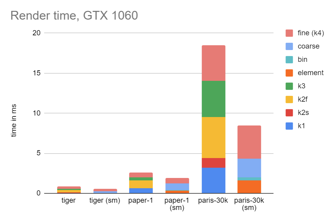
Here the timing is given in pairs, old design on the left, sort-middle on the right. These results are encouraging, including a very appealing speedup on the paris-30k test. (Again, I should point out that this test is not a fully accurate render, as stroke styles are not applied. However, as a test of the old architecture vs the new, it is a fair test).
Do these results hold up on Intel?
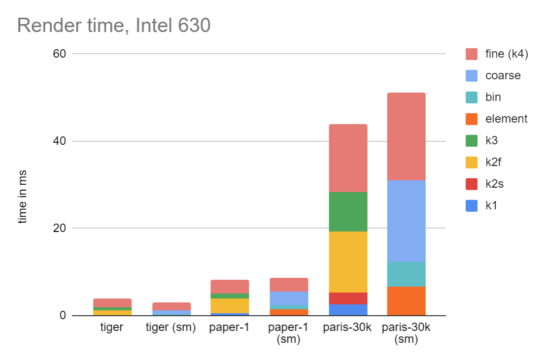
In short, no. There is much less speedup, and indeed for the paris-30k example, it has regressed. It is one of the difficult aspects of writing GPU code that different GPUs have different performance characteristics, in some cases quite significant. I haven’t deeply analyzed the performance (I find it quite difficult to do so, and often wish for better tools), but suspect it might have something to do with the relatively slow performance of threadgroup shared memory on Intel.
In all cases, the cost of coarse rasterization is significant, while element processing and binning are quite speedy.
Discussion
Performance is generally somewhat improved over the previous version of piet-gpu, but not as much as I was hoping. Why?
My analysis is that it’s a solid implementation of the concept, but that there is a nontrivial cost to carrying an element through the pipeline fully in fully sorted order. One observation is that segments within a path need not be sorted at all, simply ascribed to the correct (path, tile position) tuple. I will be exploring that in a forthcoming blog post.
Another important piece is missing from the current snapshot: GPU-side flattening. Without this, the ability to change scale in transforms is of limited usefulness, as the optimum flattening is scale dependent. Thus, the concept of “layers,” or of fonts being rendered fully GPU-side, is not yet realized. I am confident it can be implemented; in this architecture, the easiest place to insert it would be a scene-to-scene transform after element processing but before binning. It could keep sorted order either by doing a prefix sum for allocating output elements, or by atomic allocation in chunks with references to the original elements to indicate sort order.
But, these two issues aside, let’s take stock of where we are. We’ve taken a pipeline originally designed for 3D rendering, and adapted it to 2D. The pipeline itself is quite general: the core of it is just logic to pass elements in scene through to threads that work on individual tiles, with each thread given only the elements that touch that tile, and in sorted order.
The performance of this snapshot is not all bad news. One very appealing aspect is what I call “performance smoothness,” which is the absence of performance cliffs. The performance of a large number of simple paths or a smaller number of highly complex paths should be about the same, as the cost is mostly proportional to the total number of elements in the scene. An excessive number of transforms is also not a concern; these are just handled normally in the course of element processing. In the piet-metal architecture, performance was good when each node in the graph had a moderate number of children, otherwise it would degrade. And handling a large number of simple items (as might occur in a scatterplot or other data visualization) would degrade performance because each “tilegroup” does its own traversal of the scene graph. In the current architecture, early stages of the pipeline touch each element once and then efficiently send it to the appropriate bins for further processing.
As I write, I am immersed in solving the performance problems named above. Stay tuned.
I have had the good fortune of sharing ideas and analysis with Patrick Walton of Pathfinder fame as I do this work, and I am encouraged to see impressive improvements in a compute branch of Pathfinder he is developing. Pay attention to that as well.